So far I've mainly written about the fun outings and neat tours we've gone on. I'm sure you're all dying to know about why I'm really here in the first place. (Yes Mom, I actually do work).
So, the Lunar and Planetary Institute (LPI) is a NASA funded division of the Universities Space Research Association. Most of the staff here bounce back and forth between LPI and the Johnson Space Centre (JSC).
This Lunar and Planetary Summer Internship program takes students with an interest in planetary sciences from across the world to work one-on-one with the scientists at the LPI. Due to the varied nature of some of the projects, many of my colleagues do lab work at JSC.
 |
[1] Global radar view of Venus from the Magellan
"JPL must have had an excess of orange ink
the day they printed all the Venus images" |
Project topics range from meteor impact creators, lunar mapping, atmospheric modelling, mineral synthesizing, planetary surfaces and others.
I'm working with Dr. Allan Treiman, and our project is on analyzing radar properties of Venus' highlands to provide insight into surface chemistry processes.
Let me try to explain it better.
First of all, Venus is covered in thick clouds made of sulfuric acid. This makes it really difficult to see what is on its surface, because we can't take pictures of it like we do the moon or Mars. Instead, our most recent information of Venus comes from the Magellan satellite, which orbited Venus for two years, from 1992 to 1994. Even though we couldn't take pictures of its surface, we are able to use some other tools to figure out what is down there:
Altimetry - Resolution of 8x10km - Magellan was able to tell how high it was above the planet's surface,
 |
| [2]The Magellan spacecraft as it was deployed |
which allows us to produce rough topography maps.
Emissivity - Resolution of 15x23km - Measurement of how much radiation a surface emits. You can tell apart different materials by their emissivity values.
Synthetic Aperture Radar (SAR) - Resolution of 75m - Active "pinging" of Venus' surface, and measuring the intensity of the waves that bounce back
Radar is so far the best tool we have for mapping out Venus. It penetrates clouds easily, and can give pretty high spatial resolution images.
There is an established inverse relationship between elevation and emissivity on Venus, that is to say, as elevation increases, emissivity decreases. This is really interesting, because the only real variable that we know of affecting Venus' mountains is temperature. Like on Earth, it gets cooler as you go up a mountain than if you stay at sea level. On Venus, instead of using sea level (because there aren't any oceans), we use a set datum, which is mean planetary radius.
There are several hypotheses as to why emissivity might be increasing with elevation on Venus' mountain tops. One of the more popular recent theories is metal precipitation. Since Venus is really hot, it is possible that a lot of metallic compounds exist in a volatile state near her surface. As these metals cool down, they can precipitate out of the air, like when it's cold out water precipitates as snow.
Another hypothesis is that there is a mineral present that is undergoing different degrees of temperature-dependent weathering. Imagine an iron nail rusting; there are different variables that determine how quick or slow the corrosion occurs, including oxygen concentration, pH, presence of water, and temperature. Venus' atmosphere is consistent at the elevations we're looking at, so the only real factor that can control this weathering is temperature. Previous authors' have suggested that the change in emissivity is due to iron sulphides, such as pyrite, but later works have shown that pyrite is unstable. Other minerals have been suggested.
A third hypothesis is that there might be presence of a ferroelectric compound. Don't worry if that term is intimidating; it took my advisor and I awhile to figure out what was meant by that. Essentially, ferroelectric materials show a really interesting behaviour. They have a constant dielectric constant as temperature increases, until they reach a critical temperature, at which their properties spike dramatically. As temperatures continue to increase, these properties slowly decrease along a decay curve. Few minerals show are considered to be ferroelectric, making this a confusing, complicated hypothesis, but it actually fits some data quite nicely, which I will get to shortly.
My project is trying to explore this elevation-emissivity relationship, and to see if I can refine it further using higher spatial resolution data. Since we don't have any new data from Venus since Magellan, it is important to look at what we have in new ways. Emissivity is the complement to reflectivity (1-Emissivity = Reflectivity), so we decided to look at the SAR brightness instead. This gives us the resolution of 75m instead of 15x23km.
Exciting!
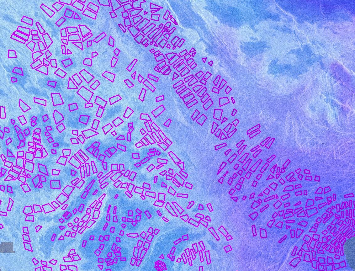 |
Example of my polygons.
Breaking the Venus-orange stereotype one map at a time. |
So, my job is to find suitable areas and to take radar brightness and elevation values to see how they compare with one another. I accomplished this by making series of polygons, and averaging out the pixel values contained within each polygon.
I didn't take the polygons arbitrarily, of course. Care was taken to avoid major faults and areas with high surface roughness. This attention to detail is what allowed us to produce a tighter graph, with less scattering.
Shown to the left and below is one of the areas I examined on Ovda Regio, one of the largest mountain ranges on Venus.
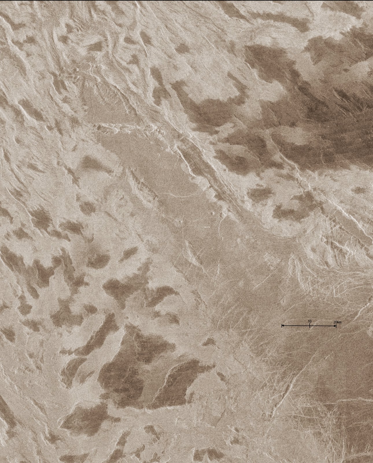 |
Essentially the same map as the colourful one,
but now you can see more of the surface topography. |
Unfortunately the scale bar doesn't show up so well, but the image to the right is approximately ~120km across.
Notable features include the smooth ramp in the middle. It extends from higher to lower elevation, and the change in reflectivity (brightness) is apparent on this image. To either side are high plateaux with some interesting dark spots on them. These dark spots are more or less at the highest elevation, and give us a unique cluster of points on my graph. Given that the emissivity data is 23km across, many of these areas were averaged out and overlooked in previous analyses. Arvidson (1994) [3] collected a few points which demonstrate the drop in radar brightness at the highest elevations, leading the hypothesis of ferroelectric materials present. We've found a few hundred of these points, supporting this interpretation.
So, here are the results:
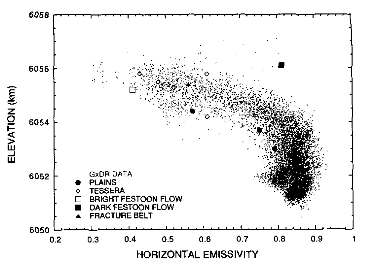 |
Previous work by Arvidson (1994). [3]
Notice that there are very few points (~6) at the high elevation, high emissivity range. |
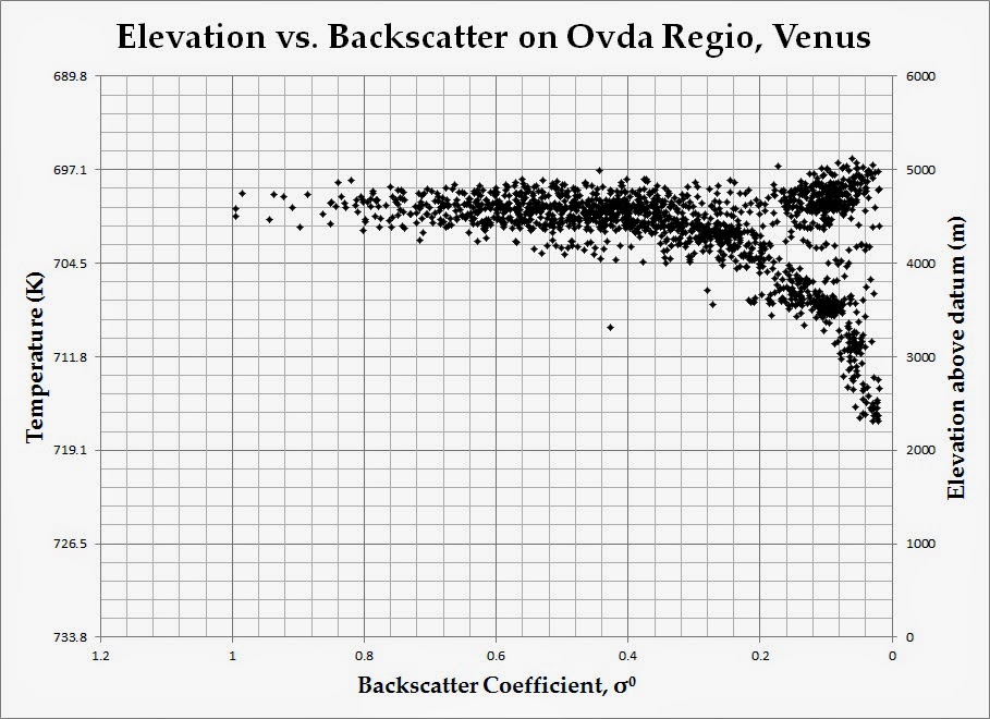 |
Harrington (2014). My graph.
Notice the cluster of points at high elevation, low radar backscatter coefficients |
So, this is pretty exciting in the field of Venus research! I finish writing up my abstract this week, and will be presenting at the intern conference on August 7th.
Cheers!
[1] "Venus globe" by NASA - http://photojournal.jpl.nasa.gov/catalog/PIA00104. Licensed under Public domain via Wikimedia Commons -http://commons.wikimedia.org/wiki/File:Venus_globe.jpg#mediaviewer/File:Venus_globe.jpg
[2]"Magellan deploy" by NASA - http://nssdc.gsfc.nasa.gov/photo_gallery/photogallery-spacecraft.html. Licensed under Public domain via Wikimedia Commons - http://commons.wikimedia.org/wiki/File:Magellan_deploy.jpg#mediaviewer/File:Magellan_deploy.jpg
[3]
Arvidson, R. E. (1994) ICARUS 112, 171-186.


