Earlier this year, Catherine and I submitted a SOAR-E proposal to acquire new RADARSAT-2 images of salt diapirs. Our original intent was to get images of halite salt diapirs in Iran to compare with our anhydrite diapirs on Axel Heiberg Island. However, we weren't able to get an images over that target site, and we needed to rethink our plan of attack. Instead, we submitted a request for four additional images over Axel Heiberg Island. One of these was over Stolz diapir, where we found halite in the field. Of our four requests, only two were granted due to RADARSAT-2 targeting conflicts. Fortunately, Stolz diapir was one of them! The other image we received is a bit north of Expedition diapir, which will provide insight into some of the discrepancies between the ASTER TIR predictions and the Harrison and Jackson field mapping.
Like with previous images, I extracted the circularly polarized data in PolSARPro, and produced terrain corrected circular polarization ratio images in SNAP. I'm pleased to say that they look great!
Here they are:
Images acquired Sept. 26, 2017 over Stolz and Whitsunday Bay diapirs.
Above, annotated HH-Intensity image. Below, CPR image.
This site was our first priority for the SOAR-E proposal, so I'm pleased it was one of the 2/4 we received. We visited Stolz and Whitsunday Bay diapirs during the 2017 field season, and samples were collected at each. Stolz diapir is where we collected samples from a halite outcrop, and has the extensive perennial springs deposits at its base. The CPR-bright spot between Stolz and Whitsunday Bay diapir to the slight west corresponds with a salt diapir we passed in the helicopter traverse between sites - I'm not sure if it has a name.
Images acquired Sept 30th, 2017. Above, annotated HH-Intensity image showing where Harrison and Jackson (2014) mapped salt diapirs, in contrast to where we observed salt signatures in the ASTER TIR images.
This site was targeted in attempts to discern the discrepancy between mapping methods. This area is subject to significant glacial coverage over the northern half, and it is likely that glacial coverage obscured the TIR signature over Expedition and Thompson diapirs. We also now have repeat coverage over Colour Diapir, which is one of the sites visited during the 2017 field season. I'm not convinced it extends as far to the west as Harrison and Jackson show. I'll need to recheck our field images.
Now here is what they look like with the 2016 images:
The Arctic DEM supports the hypothesis that the northern half of the Sept 30th image is obscured by glacial coverage
Notably, look at Whitsunday Bay diapir - it is REALLY bright in the radar image. It jumps out way more than the other diapirs. I thought for a moment that could be from early snowfall, but note that there doesn't appear to be much snow over the glacier to the west. I'll consult Landsat images shortly.
The new data is quite promising, too! Previously, the average CPR value (per pixel) over salt diapirs and secondary salts were 0.40 and 0.26 respectively. Now, once we include the new data, the average values are 0.52 for the diapirs and 0.23 for secondary salts. I'm really pleased that the new data has increased the spread between the diapirs and secondary salt deposits.
Now, on to writing, writing writing! And some XRD. But mostly writing.
RADARSAT-2 Data and Products (c) MacDonald, Dettwiler and Associates, Ltd. (year of acquisition) - All Rights Reserved. RADARSAT is an official trademark of the Canadian Space Agency. Harrison, J.C., Jackson, M.P.A., 2014. Tectonostratigraphy and allochthonous salt tectonics of Axel Heiberg Island , central Sverdrup Basin , Arctic Canada. doi:10.4095/293840
I've returned after spending some time Down Under!
This dish is 70 m across, and received the final data from Cassini
I am very fortunate to have received a grant to attend the Space Generation Congress (SGC) and 2017 International Astronautical Congress (IAC) in Adelaide, Australia. The grant was a Student Participation Initiative from the Canadian Space Agency. I love them so much.
Before arriving in Adelaide, I took a little detour into Canberra. SGC had organized an optional tour of the Canberra Deep Space Communication Complex. I knew very little about the Deep Space Network (DSN) prior to the tour, and didn't even know this site existed beforehand. The extent of my past knowledge sometimes Cassini data were lost if it was "raining in Madrid". Now I know that the NASA operates the DSN out of three facilities: Canberra, Madrid, and Goldstone (California).
I was amazed to see the satellite dish that
downlinked the final data from Cassini only days after the her final maneuver.
There were also dishes that were actively downlinking from MRO and MSL while we
were visiting – I thought that was really cool and inspiring. My first project
in planetary geology used Magellan images of Venus, and I learned that 98% of
Magellan data were downlinked in Canberra. I would like to be involved with planetary mission work in the future, so understanding the data downlink process is useful to understanding the data limitations faced by scientists in this field.
The Deep Space Communications Complex is located between granitic foothills southwest of Canberra
The SGC was an new experience for me. Instead of being a standard conference, we chose focus groups to address pressing issues in space exploration. Having a geology background, I picked the "Space Diplomacy" group, as the emphasis was on space resource mining. It was the first time I’ve been
at an conference in which I've been the only geoscientist present. This
was cool, because I was able to provide real-world
examples of terrestrial resource extracting to the discussion. It was great for
me to meet people from business, engineering and law who are all interested in
space-related topics. These are aspects of the space industry that I have had
little to no contact with in my studies, but I think might be important to know about for future career plans. SGC also hosted a cultural night, which was also a great opportunity to meet other delegates and learn about their
countries’ backgrounds and interests in space exploration. Naturally, I was thrilled that the South Korean delegates performed "Gangnam Style". We, as Canadians, brought maple cookies, maple candies, and coffee crisps to share.
Matt, one of my group mates, sketches a flowchart showing
the influences of international policy on industrial liability
and accountability.
The SGC international night was at the Adelaide Zoo. This woman is holding a bilby.
I do love any reason to dress up nice.
Moving on to IAC. I absolutely loved the
international networking opportunities and having a chance to see what space
agencies around the world are working on. The heads of agencies plenary session
was particularly great for this
because they provided an overview of the priorities and future
goals of each country. ESA gave a plenary session about setting up Moon/Mars Villages, and the vast
range of challenges associated with manned planetary exploration. I found this session interesting because many of the
infrastructural problems associated with constructing Moon/Mars Villages and in
accessing Space Resources are relevant to planetary geology.
In the exhibit hall I learned a lot about the activities
of the Japanese Aerospace Exploration Agency (JAXA), Korean Aerospace Research Institute (KARI), and ESA through the various displays and presentations. For
example, the JAXA booth hosted presentations on the status of Hayabusa-2, its
target, asteroid 162173 Ryugu, and what they learned from Hayabusa-1. Mentioned in a previous post, I worked at the Pheasant Memorial Laboratory in 2015 which was privileged to obtain some of the samples from the first Hayabusa mission, so I was curious about the fate of samples from the next mission. The KARI booth hosted a cultural event where they provided beverages and Korean snacks while talking about their recent innovations in satellite technology. I was delighted that they played K-Pop music videos while esteemed members of the aerospace industry discussed the engineering specifications of the satellites.
I think the girl group on the screen is "Twice" but I decided it wouldn't be a good use of my time at work to scour their music videos to confirm that. KARI's booth was beautifully decorated, and displayed some cutting edge tech.
Curiosity's twin hanging out in the exhibition hall
The CSA sponsored students were invited to take part in events hosted by the International Student Education Board (ISEB). At these activities, we met sponsored students from around the world. I made a bunch of friends among the KARI and JAXA sponsored students, whom I hope to stay
in contact with. One of the ISEB networking events took place in the South Australian Museum, coincidentally in the fossil/mineral/meteorite area. This was fantastic because I was able to apply my geo-knowledge and excitedly chat about minerals to anyone who was interested.
I admit that there
weren’t very many technical sessions relevant to planetary geology. I attended a few sessions on planetary
surface exploration and on remote sensing technologies, but many of the
presentations provided information outside of my area of expertise. Most of the
technical sessions I attended were aimed at an engineering audience, and even
though I want to learn more about the cutting edges of space technologies, this
wasn’t the best platform for me to do so.
That being said, I really appreciated the
multidisciplinary nature of the conferences. At IAC, I was able to see the
diversity of disciplines that contribute to space exploration, from rocket and
satellite engineering, space life sciences, government policy, astronomy and
astrophysics, Earth observation, communications, business, and public
education. I had little experience in many of these fields prior to the
congress. I feel that I now have a broader understanding of space-related
fields and how they connect with one another, and this will definitely improve
my perspective throughout my career.
At the "Women in Aeronautics" breakfast, the Director General of ESA, Jan Wörner, spoke about the importance having all types of diversity in a work place
Thesis update: I'm drying out my samples from our Axel Heiberg Island field trip. Some of the salts and soils are still a bit wet, and need to be a dry powder for doing XRD analysis.
Eclipse, 10:22 MST, I took this through a telescope
I’m writing to you after a phenomenal family vacation I took with my parents,
aunt and uncle down to Idaho and Wyoming. The main destination – the totality
zone for the eclipse! The eclipse was indeed a very breathtaking, magical
experience, but today I will be writing about some of the geology we saw. While
passing through Idaho, we stopped at Craters of the Moon National Monument. We
briefly visited with Gavin, Kevin, Raymond, and Mike who were a bit knackered
after a day of strenuous fieldwork. I won’t write much more about those lava
flows, because Gavin has written about them in stylish detail.After Craters of
the Moon, we drove into Wyoming and visited what must be a geological, volcanic
mecca – Yellowstone National Park. Now, I could write for pages about the
geology of Yellowstone, because it is such an exciting, unique place full of
epithermal wonders. For this post, I’m going to focus on two features that
seemed to show some parallels to what I saw on Axel Heiberg Island. (But you can see all my photos here!)
First are a lot of ignimbrites around the park, whose violent eruption triggered
the massively catastrophic caldera collapse 640,000 years ago. Also known as ash-flow
tuffs, ignimbrites are a type of pyroclastic flow deposits characterized by
high abundance of ash-sized (<4 mm) particles and pumice. The scale of eruption required is enough to
partially or fully empty magma chambers. The dramatic exodus of material
substantially decreases the internal pressure of the chamber, often resulting
in caldera collapse if the chamber roof is no longer sufficiently supported.
The top of the magma chamber erupts out and is deposited first, so the ash-flow
tuff sequence represents the inverted order of the magma chamber’s internal
fractionalization. The layers in ignimbrites
can be divided into pyroclastic flow units from multiple eruptive pulses. A
typical ignimbrite sequence contains a basal layer with reverse graded pumice
and lithic clasts. Above the basal layer, flow units have density separated clasts:
pumice is light and floats to the top, showing reverse grading, whereas denser
lithic clasts are normally graded. Ash-flow tuffs thin out and have fewer clasts
away from their source. If the flow units cool together, they form a compound
cooling unit. Sufficiently hot and thick ignimbrites fuse and solidify from
partial or complete welding. Welding occurs when hot, pliable pumice clasts
flatten under overburden weight and sinter together, giving them a glassy
appearance (Francis and Oppenheimer 2004).
Now you are no doubt wondering what on
earth a explosive, caldera-building volcanic unit has anything to do with salt
diapirs in the Arctic. Genetically,
nothing. But morphologically? Take a look:
The walls of this river-carved valley are jagged and karstic, looking a lot like what we saw at Stolz and Wolf Diapirs.
This looks a lot like that
pseudo-karstic topography we saw in the Axel Heiberg Diapirs. The reason is
simple. Ash, like salt, is softer than other types of rock. Therefore, it
erodes away more readily than the surrounding units and forms jagged peaks. In
fact, because ash-flow deposits are soft the Fremont First Nations used faces
of ignimbrite for wall carvings in Utah.I thought this was neat, and worthy of sharing. I imagine that ignimbrite exposed in valley or canyon walls would look very similar to salt diapirs in synthetic aperture radar, which further demonstrates the need to combine different orbital datasets paint a full picture.
Second are the hot spring travertine
deposits, like Mammoth Hot Springs. The
mechanism that forms these deposits in hot springs at Yellowstone is like the
perennial cold springs in the Arctic. In Mammoth Springs, geothermally heated
ground water passes through limestone via a fault, and leaches out calcium. The
calcium-rich water upwells to the surface and deposits calcite in the form of
travertine as it cools.
Mammoth Hot Springs has produced the largest known travertine deposit
Seismic activity alters the spring flow paths, enabling expansive terraces to form
On Axel Heiberg
Island, the waters that form Lost Hammer Spring are thought to be passing
through subsurface extents of the Wolf Diapir, thereby passing through halite
and anhydrite and leaching out sodium and calcium. Subsequently as the spring
flows over, the deposits at Lost Hammer are halite, calcite, gypsum, thenardite
and mirabilite (Battler et al. 2013). Despite Mammoth springs being a
hydrothermal system, and Lost Hammer Spring being a perennial cold spring, I
find it interesting that both sites are formed the same way.
Lost Hammer Spring, seen from above
The edge of Lost Hammer Spring, where salt-rich water has overflown and precipitated
In a week and a half, I’m going to the
Space Generation Congress and the International Astronautical Congress in
Adelaide, Australia! If I find some downtime, I’ll try to provide some short
updates here, but I’ll definitely be tweeting about the conferences!
Battler, M.M., Osinski, G.R., and Banerjee, N.R. 2013. Mineralogy of saline perennial cold spring on Axel Heiberg Island, Nunavut, Canada and implications for spring deposits on Mars. Icarus 224: 364–381. doi:10.1016/j.icarus.2012.08.031.
Francis, P.
Oppenheimer, C., 2004. Volcanoes Second Edition. Oxford University Press.
Hello,
hello, and welcome to Part II of our Axel Heiberg field adventures! As
mentioned last post, we moved campsites about half-way through the trip. The
plan was to move from Lost Hammer Spring to South Fjord Diapir. South Fjord is
the largest salt dome on the island at a monstrous 5 km diameter! We were to
make the move in three trips by helicopter. Oz and I would go first with our
personal tents and some other essential gear, the helicopter would return and
pick up a net load (literally, in a hanging net) of other gear including the
fat bikes, and then on the third trip would bring Mike and Mark with the
communal tent and the remaining gear. So Oz and I took off, needing to scout
for a place to land that would be safe, accessible, and geologically
interesting. But in a 5 km-wide mountain of continually rising and crumbling
salt, what could not be interesting?
Until we got there.
...
Oh.
That’s, um. Hmm.
Well, at least we can confirm South Fjord Diapir has rough surfaces.
There is too much snow! We can’t possibly land here! Oz is shocked – it is mid-July
and South Fjord Diapir is a winter-wonderland. He said that he visited this
site in late June some-years ago, and there was nowhere near this much snow. This
has some interesting implications for remote sensing work. Snow and ice can
heavily influence radar response – what if South Fjord dome was blanketed in
snow when our radar images were taken? I resolve to check Landsat images taken
around the dates our radar images have been taken. I have done this since
returning – it does look like one of our six images might be affected – perhaps
I should mask out the ice and snow and redo the radar zonal statistics
extraction!
What do we do? We flew around the dome for
a bit, taking pictures while deciding where our backup camp will be. Remember
that helicopter time is a valuable resource, so we need to decide quickly. Oz
asks if there is a diapir near the end of Strand Fjord. I recall that there is,
but I don’t know the distance to it. As we begin to fly over there, I pull out
the field laptop that I had in my backpack. I’ll admit, I felt pretty cool
flying in a helicopter while measuring distances in ArcGIS to make quick
decisions where to land. I determine that Strand Diapir is approximately 6 km
from the shoreline, and we deem this close enough to hike to. We’re off to land in Strand Fjord!
And oh, what a beautiful campsite it was!
Icebergs in the Fjord, a low fog is rolling through. The dark rock unit is an folded igneous sill. The brown rock is gullied the surface has undergone solifluction.
Strand Fjord, near our campsite. The sandy banks have compositional layering.
I honestly think this is the most wonderful
place I’ve ever camped. We had glaciers and ice bergs and beautiful sharp
mountains with intense solifluction. It was beautiful. I did some soil sampling
between our camp and the Fjord on one of our off days. Again, we saw patches of
precipitated salts. Interestingly, these salts tended to be concentrated along
the rims of wet/dry sand boundaries. The whole fjord area shows up in the TIR
images as having VERY STRONG gypsum/anhydrite signatures, all deriving from the
nearby Strand Diapir. Mike, Mark and I went on a hike to visit the northern
half of the diapir exposure one day. The inland-area of the Fjord appears to be
a glacially carved U-shaped valley, so Strand Diapir is split into two main outcrops
across the valley. The salts in Strand Diapir are also
interacting with some volcanic intrusions, causing some beautiful iron
staining.
Behind me is the glacier that carved the U-shaped valley and provides the meltwater for the river.
The brilliant colours are from oxidation reactions between igneous rocks and the diapir. The igneous rocks provide the metals, the anhydrite provides sulphur.
A reoccurring theme, the outcrops show some exposures of intact rock
salt, but the majority of the surface has weathered into the highly vuggy
gypsum crust that is characteristic of the Axel Heiberg Island anhydrite diapirs.
Part way up the valley wall, the anhydrite is interbedded with what I think is
limestone. I haven’t exampled the sample yet, but the dark colour and texture
looks like a carbonate and past literature states that limestone is commonly
interbedded with the Otto Fjord Formation salts. On a regional scale, the
diapir material is stratigraphically overlying the orange stained unit, which I
think is a volcanic sill, and has since undergone synclinal folding.
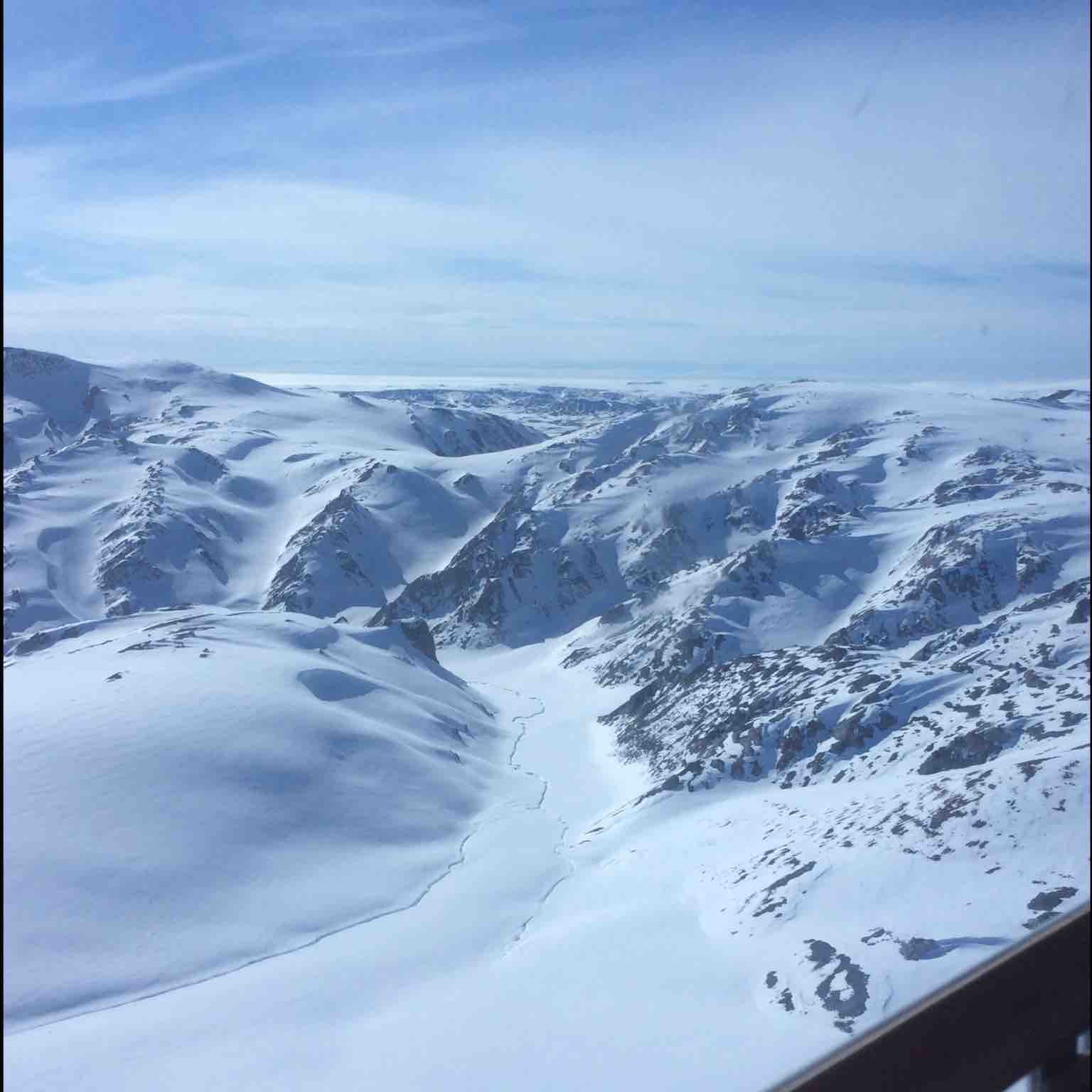
Flying in a helicopter never gets old
Something that I really appreciated this
trip was being able to finally investigate the mystery of the radar-dark bright region,
mapped as Isachsen Formation (quartz sandstone with some igneous intrusions).
As a weather front was rolling in, our helicopter pilot asked if we wanted to
make any last quick visits. I gave him the coordinates at the centre of the
feature – the peak of a broad mountain range. He looked westward, and observed
that that was where the storm was the thickest, and he wouldn’t be able to land
there. Nonetheless, we headed that way along the coast, wary of the thick
clouds in the distance. The very peaks were shrouded in clouds, but he asked if
seeing the sides were enough. Elated to be there, I said yes, and to my delight
we made a full perimeter tour around the feature before heading back to the
safety of our campsite. Many photos were taken, and the verdict is that these
slopes are COVERED in cobble-sized talus that would effectively scatter
RADARSAT-2’s 5.6 cm radar beams. Since these are also high elevation peaks,
snow and ice is admittedly also a possibility. I’m going to check the Landsat
images soon to investigate. Sadly because we couldn’t land I wasn’t able to
sample, or get good scaled photos. -sobs-
In addition to the fist-sized rocks everywhere, take a moment to appreciate that sweet folding.
Travertine terraces from perennial spring from Colour Peak
Finally, one of the highlights of the trip was scaling the
550 m Colour Peak. Colour Peak has been part of the epitome for my thesis, showing that salt diapirs are radar-rough, whereas the materials that erode off of them and reprecipitate elsewhere are radar-smooth. Mark and Mike spent the day sampling the calcite-rich perennial
springs effusing from the base of the mountain. The springs are building terraces
of black travertine – the type of calcite that precipitates from cold water
springs. 1-3 mm cubic halite crystals lined the edges of the streams. Mike
founds some really cool crystals in a small cave – the sample he gave me is
decorating my coffee table as I write this. The smell of H2S was
pungent, and I found myself craving egg salad whilst down there. Oz and I,
however, journeyed up to climb the massive diapir. The best exposures of salt textures were at
the top, with the flanks being either covered in soil, talus, or completely
weathered and crusty outcrop. The ascent
was tough. The diapir is steep sided
covered in poorly sorted colluvium. The skree contains sand to boulder-sized
rocks. We also found some palm-sized fragments of clear selenite crystals
amongst the soil patches. I think the anhydrite colluvium and gypsum-rich soil
is enough to product the spectral signature seen in the ASTER TIR image
downslope of Colour Peak without us needed to appeal to the perennial spring. Because
much of the slope material was unconsolidated, our feet were prone to slipping
down as we moved upwards. I’m very fortunate that Dr. Osinski is an experienced
climber, and I was able to follow where his footsteps packed down the debris. Frequently we would take a step on what
seemed to be solid ground, only to have our foot punch through the weathered
gypsum crust into a 20 cm deep vug.
Rough, steep, the return of slightly karst-y topography.
Close
to the summit are outcrops of solid anhydrite or gypsum. Unlike at Wolf Diapir,
where the solid salt was powdery and friable, here the salt is
crystalline. Erosional processes are
carving the solid salt into points like the rillenkarren seen on halite diapirs
and in karstic carbonates. The rillenkarren are smooth at the mm scale, but
undulate at the cm scale and would appear rough at C and L-Band SAR.
Rippled rillenkarren textures on crystalline anhydrite sample.
The sharp,
solid salt looks beautiful up close. Of
course, nothing compares to the stunning, beautiful view from the summit!
Yes.
An excellent view across Expedition Fjord, and the travertine perennial spring down below
Wow.
The rocks up here are mostly blocky, partially weathered, and the ground is
covered in colluvium. Once again we are able to confirm that salt diapirs are
rough on the ground, not just in radar.
Very blocky, rough, and sadly too unstable and dangerous to venture farther.
You can see where Colour Diapir ends, and the adjacent mountain begins based on surface texture alone.
Any
discussion of Colour Peak would be incomplete without explaining how it got its
name. The colluvium also includes rubble and gravel of angular igneous
lithologies, including what is ostensibly dacite and diorite. Some of the
volcanic material is oxidizing to form gossans. The gossans are dazzling zones of
vivid orange, yellow, and brown alteration. These are found in close
association with diapirs on Axel Heiberg Island, including North Agate Fjord
and Junction Diapir where basaltic intrusions from the Isachsen Formation are
altering to form copper and iron sulphides and secondary copper sulphates
(Williamson 2011). The calcium sulphates in the diapir provide the sulphur for
these alterations to occur. Remember, we saw this same alteration at Strand
Diapir! We collected some samples of
yellow rhombohedral crystals have been taken to the lab to for analysis
The journey home was bittersweet. I’m going to miss this place.
And such concludes my 2017 Axel Heiberg
adventure.
Okay, now that I’ve
had a week to recover and sort through things, I am delighted and excited to
share some of my field experiences with you!
July 5th-20th marked a two-week adventure into the
Canadian High Arctic. Our goal: Axel Heiberg Island. This is why this blog is called, “Arctic
Resolution” after all! In a sense, this trip is the epitome of my M.Sc thesis
because it gave me the opportunity to “ground-truth” all the observations and
analysis I’ve been doing remotely up to now. In essence, I got to see what my
radar and spectroscopy images look like in person! It was seriously cool to be
able to have that opportunity.
If you need to recap quickly what my thesis is about you can watch me explain
it in three minutes:
We are trying to
see how radar can be used for remote predictive geological mapping. Remote
predictive mapping is not only useful on Earth to save time and money – it is
often the only way we are able to learn about the surfaces of other planets and
moons. The techniques we are developing are important for planetary science, as
Earth is the only planet humans like us can go and check in person. Thus the
need for terrestrial analogue studies, which is one of the focuses and
strengths of the University of Western Ontario’s Centre for Planetary Science
and Exploration. My project is largely grounded in economic geology (salt
diapirs -> petroleum + ore deposits -> $$$ = 😊), but
I like that this project also has potential analogues for radar mapping and is
helping me develop skillsets vital to planetary sciences.
So, what did we see?
~~~LOTS OF FUN THINGS~~~
This blog post, for the sake of avoiding
rambling on and on, will contain summaries of Part I of our field adventures.
About half way through our time on Axel Heiberg we moved campsites from Lost
Hammer Spring to Strand Fjord, so I will cover our work done around the first
campsite.
We found one of
our first scientific findings before the Twin Otter even landed. Remember how I
was puzzling over the nature of secondary salts? The strong ASTER thermal infrared
spectral signatures for gypsum or anhydrite that weren’t confined to salt
domes, but rather in gullies and river floodplains? I was wondering if those
signatures were the result of:
1. Rubble and gravel of
mechanically eroded diapir materials (chunks of salt rock)
2. Precipitated salt
minerals that geochemically dissolved out through water flow
Number 2 is our winner! Just looking out
the Twin Otter windows the secondary, precipitated salt is abundant and
widespread.
Salt minerals precipitating in gullies and floodplains
Of course, we confirmed that it is salt minerals on the ground
later, and have collected many samples that we will XRD to identify, but it is
incredible that we solved one of our biggest field objectives before even
landing! These hillslopes and floodplains are predominantly radar-smooth soils,
with some colluvial or fluvial pebbles and cobbles. The salt bearing gullies and stream channels
contain larger pebbles, cobbles, and sporadic boulders, but I think these
features are too localized to affect the CPR images at the scale of RADARSAT-2
or PALSAR-1 multilooked CPR image resolution. The salt encrustations are <1
mm in thickness on the surfaces. Although boulders and cobbles of salt have
mechanically broken off diapiric structures, like the flanks of Wolf Diapir,
these likely contribute to the rougher radar signatures seen in the CPR images
in association with the diapirs. Later, I also found that there are at least
two types of salt minerals precipitating: halite, and what is likely gypsum or
anhydrite. I discovered the halite using the classic method all new students
learn in Earth Science 101 – licking the samples.
However, what sort
of surprised us was the weather-dependence of these surficial salts. When we
first arrived, on a beautiful, clear, sunny day, these salts were very sharp in
contrast against the landscape. When I walked up the stream at our first
campsite, the rocks in the riverbed exposed above water were coated in a white
crust. Then the rain and snow came. After three days of snow, almost all of the
white encrustations disappeared! There were still white patches on the
hillslopes and in gullies, but they weren’t nearly as stark as before. After a
day or two of the weather clearing up, the white minerals appeared again,
almost as abundant as when we arrived. We think the snow and rain dissolved the
salt minerals and they were able to precipitated again from the surface water
after the ground was able to start drying.
Salt minerals encrusting some rocks on hillslope
Our first campsite
was at Lost Hammer Spring. Lost Hammer Spring is a perennial spring, one of
many places on Axel Heiberg Island where brines upwell to surface and deposit
large precipitated structures of salt. It is entirely possible that the source
of the salt in these fluids derives from the core of the adjacent Wolf Diapir,
but this has not been conclusively proven. The salt that makes up Lost Hammer
is very sodium rich, implying that the groundwater has interacted with
subsurface halite (i.e. table salt) (Battler et al. 2013) but no halite has yet
been found at Wolf Diapir. The only diapir at which halite has been found is at
Stolz Diapir, which we visited and sampled later in the trip. It is entirely
likely that many diapirs on Axel Heiberg Island contain halite in their cores,
and that this is simply not exposed at surface. Curiouser and curiouser! Halite
was even found precipitating in small patches a few kilometers downriver from
Lost Hammer. Like the secondary salts, Lost Hammer Spring exhibited a similar
wet/dry cycle. Upon arrival to the field site, the Lost Hammer Spring was a
dazzling white, but during the snowfall the spring became greyer and muddier.
Either the surface layer of salt was exfoliated, or mud was transported onto
the spring during the wet interval.
Not a snow bank, this is all salt! Lost Hammer Spring (aka Wolf Spring) has accumulated an almost 2 m high vent of halite, calcite, gypsum,
thernardite, and microbilite. The shape of the perennial spring changes seasonally, with periods of partial dissolution and reprecipitation
Wolf
Diapir is characterized by having steep slopes and heavy erosion compared to
surrounding rocks from the Isachsen Formation and the Invisible Point Member of
the Christopher Formation. The contrast in surface texture is sharp between
Wolf Diapir and the other formations. Whereas the adjacent rock formation has
regularly distributed gravel in soil, the flanks of the Wolf Diapir are characterized poorly
sorted very angular colluvium from sand to block sized particles. Two textures were pervasive amongst all the diapirs we visited this trip - solid, crystalline anhydrite, and weathered, heavily altered vuggy gypsum.
Wolf Diapir. You can see how the surface of the mountain is far rougher and more gullyied than the surrounding hills.
Close up, you can see how heterogenous and blocky the surface of the diapirs are. Broken fragments range from granule to block sized. It is frequently difficult to determine which blocks are in situ or broken
This weathered, vuggy crust is pervasive across all diapirs we visited.
Other intact anhydrite (or gypsum?) has different lithologies across different diapirs.
At Wolf, the crystalline material was very friable (likely still altered) and highly veined with what might be limestone.
A long gully
with 2 m high levees made up of large angular boulders runs down the eastern
flank of the structure. We mapped this using a portable LiDAR system.
Dr. Osinksi stands adjacent to the 2 m high colluvial levee flanking a prominent gully coming down Wolf Diapir
On one of our helicopter traverse days, we could visit Stolz and Whitsunday Bay diapirs are located outside of the WABS region, on the eastern side of the island. Right now we don’t have RADARSAT-2 or PALSAR-1 coverage over these sites, but I contacted a gentleman at the CSA about using our SOAR-E proposal to get some. For now, we are interested in their chemistry and spectral responses. The top of the diapir is encrusted with a thick, weathered crust of gypsum/anhydrite. The slopes are steep, with large blocks broken off on the flanks and in the valleys. The topography on Stolz Diapir is karstic, with tall, jaggaed pillars of eroded diapir material.
In some places, the erosion characteristics of Stolz Diapir appeared karstic in nature.
We saw some of this later on at Colour Peak as well.
Like Wolf, Stolz Diapir is very rough and blocky.
Large vugs within and beneath the altered crust and small dissolution caves run
throughout. Two streams run through the structure, converging along the eastern
flank. These two streams have different water chemistries and sediment load.
One stream has distinctively more halite than the other, and likely runs
through Stolz’s halite core. Halite is exposed in outcrop downstream of where
the streams converge. Textures within the halite range from white powdery
massive structureless to colourless/grey clear crystalline halite with perfect
cubic cleavage. Some areas of crystalline halite are green tinged from
localized yellow spots which may be endolith colonies.
Dr. Osinksi stands in front of large halite outcrop
In certain places, the halite could be seen growing in framboidal bulbs of small cubes
There are extreme,
extensive, thick perennial springs deposits downstream. They are seriously insane. It looks and feels
like walking through snow! These salts have varying textures, colours, banding,
and crystal structure. Upstream are alternating light and dark grey salts.
Downstream by a pool are pure white, snow-like salts with bladed/rod crystal
structures. The strength of anhydrite/gypsum over the spring deposits is
notably weaker than the signature over the diapir itself, likely because the
spring is predominantly formed from precipitated halite or calcite travertine.
Extensive, massive perennial springs! The white and grey is all salt!
Note the differences in colour and texture between the white and grey salts.
Mark sampled each, and so hopefully he'll be able to tell us what they are.
Salt salt
salt! Everywhere! So that concludes the
first part of Arctic updates. Stay tuned for part II within the next fortnight.
Last post, I mentioned that I would provide a recap of the Earth Observation Summit in Montreal, June 20-22th. I am very happy to have had the chance to both learn about up and coming earth observation technologies, as well as present my own research at the summit. Admittedly, you, dear readers, are probably more interested in hearing about my Arctic Adventures to Axel Heiberg Island (July 5th-20th), but I haven't quite sorted through my notes and photos from the trip yet to write a blog post about it. Soon! Likely for next week.
I had the pleasure of attending both the Synthetic Aperture Radar (SAR) Workshop and the Summer School. During these seminars, we learned about different applications of SAR, types of hyperspectral remote sensing, and the use and application of unmanned aerial vehicles (UAVs) for research, military, and civilian purposes. Something that really stuck out to me was the level of resolution and detail attainable from hyperspectral analysis. I knew that spectroscopy could be used to differentiate rocks, mineral content, vegetation, and man-made structures as I have done similar classification in remote sensing coursework and for my thesis. But at the workshop I learned that "level three" hyperspectral imaging can be used to differentiate between specific types of plants and roofing materials of buildings. This surprised me, and I'm really impressed by the versatility of spectroscopy, and all the fields it can be applied to. I suppose it makes sense, I mean, if spectroscopy can differentiate between different minerals, why wouldn't you be able to detect different types of plants and polymers? I never thought about it. In a different session, I also learned that the spectral signatures of plants are seasonably variable based on phenological changes. This is intuitive, since plants go through different phases of growing, leave production, and leaf loss, but again, it is something I hadn't thought about.
Before the SAR Workshop, I knew radar had a variety of applications in ground subsidence, natural disaster monitoring, and military intelligence, but did not know the nuances behind how these techniques were applied. Now I have a better understanding of the many Interferometric SAR processing steps for monitoring ground movements, and how RADARSAT-2 is used for naval surveillance in the Canadian Arctic.
My presentation “Polarimetric radar for remote geological mapping of salt diapirs on Axel Heiberg Island, Nunavut” was well received in the Polarimetric SAR Processing session. The session was well attended, and some audience members asked insightful questions about my work. One gentleman asked if we were potentially detecting limestone in addition to gypsum and anhydrite with our Advanced Spaceborne Thermal Emission and Reflection Radiometer (ASTER) spectroscopy and in our radar images because both limestone and gypsum can show similar signatures. This is another case of where radar and topographic information may be useful in differentiating the differences between different rock lithologies based on their morphology and surface textures. I am delighted and honoured to say that my talk won second place for “Best Student Presentation” at the Congress. I am always happy to talk about rocks and satellites, and would love the opportunities to continue to share my knowledge and research in salt diapirism and polarimetric radar remote sensing at future conferences and meetings. Anyone who has been around me in the past few months has probably heard my three-minute thesis half a dozen times as I elucidate new quarry about the wonders of remote predictive mapping.
Over the course of the congress, I had many opportunities to connect and reconnect with colleagues and industry professionals. It was a pleasure to speak with representatives from the Canadian Space Agency again after meeting them last November for the Mars Sample Return Simulation at the University of Western Ontario. I also reconnected with people I had met at the Canadian Space Exploration Workshop whom I discussed the status of the RADARSAT Constellation Mission. Since I've been using RADARSAT-2 data for my thesis, I'm curious about the coverage the Constellation Mission will provide improved coverage over the Canadian high Arctic. I also met one of the Advisory Board members for the Students for the Exploration and Development of Space (SEDS-Canada) for the first time that I had been in contact with through e-mail. I'm currently the Vice-Chair of SEDS-Canada, and working with the Board of Advisors is one of my roles in that.
In summary, the Earth Observation Summit was a very productive meeting. I learned a lot about SAR, which is beneficial to my M.Sc. research work, as well as other methods of remote sensing that has given me a more well-rounded and diverse understanding of Earth observation methods. I met many satellite industry professionals and learned a lot about Canada’s contributions to the space industry. This opportunity has given me a broader global understanding of space systems sciences. I look forward to being able to apply what I have learned at the Summit towards my future career aspirations in planetary mission work and space administration.
Soon you will hear about my Axel Heiberg adventures. Soon.
I'm very excited to say that next week I have the pleasure of attending the Earth Observation Summit in Montreal! The summit is a combination of three meetings: the 38th Canadian Symposium on Remote Sensing (CSRS), the 17th Congress of the Association Québécoise de Télédétection (AQT) and the 11th Advanced SAR (ASAR) Workshop. My main purpose in attending is for the ASAR Workshop, but I am also very keen on learning all about the cutting edge remote sensing techniques and satellite technologies!
I have a presentation in one of the sessions on Advanced Polarimetric Methods. Mike and Hun will also be attending, and they have talks in the Geology session (wah! I'm geology, too! But my topic fits in either session :) ) Next post, I'll tell you all about the cool things I learned!
In preparation for my talk and our upcoming field season to Axel Heiberg Island, I was going through some of my data with a fine picked comb. Remember those PALSAR Hiccups I was having before? It turns out things are a bit worse than I previously thought! Not only are the images poorly registered (i.e. they don't line up with the other maps properly) but there is also some severe distortion to a process called 'layover', which is a common, unfortunate challenge with radar imaging. I wrote a little bit about layover in a previous post last year. Usually terrain correction helps lessen the distortion.
Compare these HH-Intensity image pairs:
Figure 1 Two images of South Fiord Diapir. Above, RADARSAT-2, water is masked out. Below, PALSAR-1 with water included. Note how the shape of the dome is distorted in the PALSAR image, with a thick white line on the eastern margin.
Figure 2: Above, RADARSAT-2, below PALSAR-1. Again, water is masked out in the RADARSAT but not the PALSAR image. Pink outlines delimit salt diapirs as identified in other spectral datasets, including (west to east) Surprise Central Diapir, Bastion Ridge Central Diapir, and Glacier Fiord Diapir. Notice how the mountains are more defined and '"3D" looking in the top image, but appear almost sideways or overturned in the lower image. Additionally notice how combination of the layover distortion and poor image registration results in the pink outlines being offset from the actual features.
The cause for this distortion is the incidence angle. The incidence angle is the angle between the radar beam and the normal (perpendicular to) to the surface (Figure 3).
Figure 3: Illustration of angle of incidence, from Wolfram
For the RADARSAT-2 images the incidence angle is ~40▫, where as the PALSAR-2 images have an incidence angle of 21.5▫. For a flat surface, this wouldn't be much of a problem. However, as shown in Figure 2, Axel Heiberg Island has a lot of hills, mountains, and diapirs! The angle of repose for most materials is around 30▫, and that can be less for bigger blocks. It is likely that a lot of the mountainous areas are sloping close to the incidence angle of the PALSAR-1 images. This means that the radar beams are inflicting the surface almost perpendicular to the mountains, making them look flat! And oddly sideways! To help me visualize this better, I made some sketches and set up a physical model using my bus pass, an external hard drive and a pen, but hopefully you won't need to do that.
There are two main types of slope angle effects, forshortening and layover. Most radar images (unless you are looking at extremely flat terrain!) will experience these to some extent. The effects are exacerbated in mountainous areas, and with smaller incidence angles. Recall how radar works - we are sending a beam to a surface, and measuring the amount that bounces back. The amount of time it takes for the beam to bounce back can affect its position in the image, so if a radar beam is taking different amounts of time to reflect off of different parts of an object, that can affect what the object looks like in the image.
Foreshortening occurs with a radar beam reaches the bottom of a slope feature before the top. In foreshortening, slope facing the radar beam will appear "shortened" in the resulting image. The lower image in Figure 1 shows foreshortened western flank of the diapir dome. Layover is similar, but occurs when the radar beam hits the top of the slope before the base. This makes it look like the sloped feature is tilting towards the radar position. The lower image of Figure 2 is a better example of layover, because it looks like those mountain ranges are tilted sideways towards the east (I think - that's what it looks like to me, but I'm still learning how to recognize these effects. :) )
Ultimately, these distortions have shown that not all of our PALSAR-1 data is reliable. I noticed that a lot of the salt polygons were misplaced from the distortions. However, I am happy to say I was able to perform a quick band-aid solution. I went through each of the polygons and did a quick visual assessment to see if the radar looked reliable. I manually moved some of the polygons in ArcGIS so they would be overlying the right features even if the shapefiles aren't registered the same. This has given me enough patched-up data to still present some PALSAR-1 results at the conference next week, but it is a short term solution until we either re-register the data, or scrap it.
So, the 'new' results show that the salt diapirs more rough in PALSAR-1's L-Band than in C-Band. In C-Band, the CPR average values are ~0.4, but in L-Band they are ~0.6! The non-diapiric salts have similar signatures. In C-Band non-diapiric salt has CPR ~0.21, and in L-Band it is ~0.23. Previously we thought there were some radar-rough areas of non-diapirc salt in L-Band, but I have confirmed those were registration issues.
This is still good, and we can work with this!
I'll let you know how the Earth Observation Summit goes!
For more information on radar slope effects, this page is awesome:
RADARSAT-2 Data and Products (c) MacDonald, Dettwiler and Associates, Ltd. (2016) - All Rights Reserved. RADARSAT is an official trademark of the Canadian Space Agency.