$ pwd
Elise
$ ls
Body Mind
$ cd Mind
$ ls
Things I know Things I don't know
$ cd Things I know
$ ls
Geology K-Pop Baking Philosophy World Mythologies
$ cd ..
$ cd Things I don't know
$ mkdir Linux
$ cd Linux
$ cat > Line_Commands.txt
Tuesday, June 28, 2016
Monday, June 20, 2016
Summary of rock formations on Axel Heiberg Island
This information was compiled with Rachel Maj and Maria Shaposhnikova. Summaries are from Harrison and Jackson (2014). This post will be continually updated as we develop a better understanding of the Axel Heiberg strata, and the significance each of the units plays in studying diapirism on the island.
(Written in order of depositional history, oldest at the top)
Borup Fiord Formation
Intrusive igneous rocks
Strand Bay Formation
(Written in order of depositional history, oldest at the top)
Borup Fiord Formation
- Early to Late Carboniferous
- Thickness ranges from 40 - 1100 m.
- Northern Axel Heiberg Island
- Red weathered Quartz Sandstone + Polymictic conglomerate
- Minor Arenaceous Limestone
- Locally abundant non-marine carbonate
- Interpreted as proximal alluvial fans grading into stream channel, braidplain, overbank on distal alluvial fans
Otto Fiord Formation
- Early to Late Carboniferous
- Up to 410 m thick
- Source of all evapouritic diapirs in central Sverdrup Basin
- Stratified, 8-50 m thick Anhydrite and Limestone cycles, rare dolostone and sandstone
- Diverse fossils present in limestones
- Localized brecciation
- Sparse halite on Axel Heiberg
Hare Fiord and Trappers Cove Formations
- Late Carboniferous
- Up to 1200 thick combined
- Siltstone, Shale, Siliceous Shale, Spiculitic Chert, Limestone
- Exposed on northern and eastern Axel Heiberg Island
- Strata occurs in incomplete Bouma cycles
Van Hauen and Black Stripe Formations
- Lower to Upper Permian
- Combined thickness between 180 to 360 m
- Result of sediment starvation
- Dark, fissile shale, dark siltstone, dark chert. Rare limestone
Blind Fiord Formation
- May be between 1000-1500 m thick
- Siltstone and shale, some red weathering
- Soft sediment deformation, cross bedding
- Annelid worm tracks (Zoophycos?)
- Late Permian to Early Triassic
- Contains cretaceous gabbro sills that conformably overlie the Van Hauen Formation
Blaa Mountain Group
- Contains four formations: Murray Harbour, Buchanan, Hoyle Bay, and Barrow Formations
- Dark shale, weathered siltstone, sandy siltstone
- Clay ironstone concretions
- 245.9-203.6 Ma
- Thin towards diapirs
Heiberg Formation
- Three members Romulus (pale sandstone, siltstone, shale, coarsening upwards cycles) Fosheim (light sandstone, less siltstone, carbonaceous shale, coal interbeds) Remus (light sandstone, quartz and iron cement, clay)
- Red weathering - iron likely comes from Fosheim member
- ~331-1422 m thick
- This formation is important evidence for the salt diaprism
Savik beds
- Composed of the Jameson Bay Formation, Sandy Point Formation, McConnell Island Formation, and Ringes Formation
- Lower Jurassic
- Dark grey to black shale, glauconitic shale and sandstone - Formations are grouped together because they are not possible to distinguish outside of the hand sample scale
- 270 m to 819 m in thickness
Awingak Formation
- Quartzose sandstone and shale
- Approximately 345 m thick
- Plant debris, coal, roots
- Thins by more than 50% adjacent to diapris
- Hornfels and breccias
- 161.2-161.8 Mya
- Debris flows
- Lots written about this - might be relevant to return to
Deer Bay Formation
- Kimmeridgian to mid-Valanginian (Late Jurassic to Early Cretaceous)
- Silty shale, clay ironstone interbeds, black silty shale
- Characterized by presence of glendonites
Isachsen Formation
- Valanginian to Aptian (Early Cretaceous)
- 92 to 1372 m in thickness
- Light quartz sandstone with lesser carbonaceous siltstone, shale and coal
- Coarsening upwards cycles
- Contains the Rondon Member (coarsening upwards cycles of shale, siltstone, bioturbated sandstone), the WalkerIsland Member (coarsening and fining upwards cycles of sandstone, carbonaceous siltstone and shale)
- Some mafic sills
Christopher Formation
- Dark shale and silty shale, minor siltstone, and very fine grained sandstone
- Total range in thickness 343 to >2100 m (including areas of thinning and minibasins, but generally 442-1100 m
- Early Cretaceous
- Splits into the Invincible Point Member and the McDougall Point Member, members are separated by the Junction beds at top of Invincible Point Member
- Invincible Point Member - lower 645 m of formation, dark silty shale, some ironstone and calcareous mudstone concretions, glendonites, petrified wood. Interbeds of sandstone, tuff, and siltstone, contains stratified anhydrite
- Junction beds - up to 60 m thick, coarsening and thickening upwards cross-bedded sandstones to the north
- Macdougall Point Member - dark silty shale, with siltstone and fine sandstone, concretions and petrified wood, 210-550 m
Hassel Formation
- 80% Sandstone, 20% shale, 5-20 m coarsening upwards cycles at Expedition Fiord
- Sandstones are medium grained calcarrious and dolomitic arkose and subarkoses at E
- 105 to > 500 m thick
- Covered by basalt and other mafic talus
- Early Cretaceous
Bastion Ridge Formation
- Early Cretaceous
- Shale, siltstone, minor thin beds of sandstone and sideritic ironstone
- 5-242 m thick
- Contains mafic sills and volcanic flows
Strand Fiord Formation
- Early to Late Cretaceous, may be conformable and contemporaneous with the Kanguk Formation
- Sucesssion of basalt, agglomerate, and pyroclastic deposits
- 40-1033 m thick
- Flows are 15-60 m thick
- Flow tops are vesicular and amygdaloidal
- Flows have aa, pahoehoe, and blocky textures
- Some hyaloclastic flows, ash-fall deposits and fluvial conglomerates
Intrusive igneous rocks
- Mafic
- Coarse to medium grained (gabbro-diabase)
- Dyke swams, including the Queen Elizabeth and Surprise dyke swarms (Surprise! It's a dyke swarm!)
- No strong relationship between age, trend, and stratigraphic level of emplacement
- Older dykes may have facilitated flows in younger units
- Early Creataceous - Ages of dykes are not well constrained at the Age level
Kanguk Formation
- Late Cretaceous
- Thickness between 31-847 m
- Dark shale, interbeds of sandstone and siltstone
Expedition Formation
- Late Cretaceous
- Comprises a lower and upper member
- Lower member is 160-947 m thick
- Lower member is ~60% shale, ~40% sandstone
- Sandstones in Lower member contain planar tabular cross-stratification, ripples, plant fragments, bioturbation, and is organized in both fining and coarsening upwards cycles
- Upper Member is 0-746 m thick
- Upper member is sandstone and shale in coarsening upwards cycles
- Upper member sandstone is medium to coarse grained cross-bedded sandstone
- Upper member grades into shale and carbonaceous shale to the west
- Upper member contains pebble lags
Strand Bay Formation
- 53 to 783 m thick
- Paleocene
- Shale dominated, with sandstone interbeds
- Coal seams
Iceberg Bay Formation
- Paleocene to Eocene
- Composed of the Lower Member and the Coal Member
- Full description in Ricketts (1991)
- Lower Member consists of 30-50% sandstone, shale, and coal
- Lower Member is up to 1838 m thick
- Lower Member consists of 15-45 m coarsening-upwards cycles
- The Coal Member is well preserved
- The Coal Member is up to 1060 m thick
- The Coal Member contains 1-10 m beds of fining upwards sandstone, coal, and shale
- The Coal Member contains fossil wood, lags of mud chips, and leaf imprints
Pleistocene and Holocene Sediments
- Gravels, Diamicts (till)
- Authors provide interpretations rather than unit descriptions
Jackson, M.P.A., and Harrison, J.C., 2006, An allochthonous salt canopy on Axel Heiberg Island,
Sverdrup Basin, Arctic Canada: Geology, v. 34, no. 12, p. 1045–1048, doi: 10.1130/G22798A.1.
Friday, June 17, 2016
Sentinel-1 Toolbox Tutorials Part 2: Interferometry
Hello everyone, and here is part two of my overview of the ESA's Sentinel-1 Toolbox tutorials. This entry is following the terrain corrections tutorial, which also uses RADARSAT-2 data. This time we are looking over Phoenix Arizona.
Interferometry is a technique that creates a an image that does awesome cool things! One application of interferometry explored in this tutorial is the ability to use interferograms to produce DEMs or topographic phase bands. A similar application will be applied when I work towards my end goal project. Remember those salt diapirs from the last post? We will be using InSAR from different time intervals to check their height, and determine if they are moving (and if so, at what rate!)
For all intents and purposes, my M.Sc thesis is to tell the Canadian Space Agency to fire radio waves at squishy salt rocks in a polar desert, and then see how much they are oozing out of the sedimentary basin. That is pretty great.
The tutorial starts us off with a set of Single Look Complex (SLC) radar images over Phoenix, Arizona. We need to select the band we are working with, and coregister the images.
Next, we are able to generate an interferogram from the coregistered images. The computer does some slightly intimidating trigonometry for us, but clicking on the tools in the program is pretty easy.
The space between two fringes of the same colour represents a 2pi cycle, which is half of the sensor's wavelength. This means that the closer together the fringes, the greater the topographic variation.
In producing the interferogram, we also produced a Coherence Band which shows how similar the master and slave radar images are.
For all intents and purposes, my M.Sc thesis is to tell the Canadian Space Agency to fire radio waves at squishy salt rocks in a polar desert, and then see how much they are oozing out of the sedimentary basin. That is pretty great.
The tutorial starts us off with a set of Single Look Complex (SLC) radar images over Phoenix, Arizona. We need to select the band we are working with, and coregister the images.
 |
| One of the radar images of Phoenix, Arizona |
 |
| Interferogram of two radar images |
In producing the interferogram, we also produced a Coherence Band which shows how similar the master and slave radar images are.
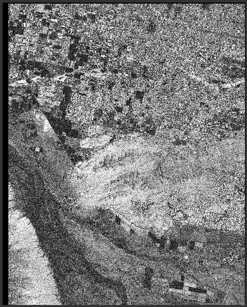 |
| Coherence Band - Dark areas have poor coherence (like vegetation, which is variable between the two images) whereas buildings have high coherence (they move less) |
There is a tool we can use to "flatten" the interferogram (i.e. remove the fringes in relatively flat areas, and smooth out the topographic phases). This tool removes the topographic phase, and effectively produces a DEM out of the interferogram.
Alternatively, there are other filtering processes we can implement on the interferogram. One way of reducing noise from temporal decorrelation, geometric decorrelation, volumetric scattering, and general processing errors through unwrapping. Before we can unwrap the phases, we need to apply the Goldstein Phase Filtering process. You will notice that the Goldstein filtering increases the intensity and contrast of the interferogram fringes.
 |
| Topographic Phase Band - We produced a DEM through interferometry! |
Alternatively, there are other filtering processes we can implement on the interferogram. One way of reducing noise from temporal decorrelation, geometric decorrelation, volumetric scattering, and general processing errors through unwrapping. Before we can unwrap the phases, we need to apply the Goldstein Phase Filtering process. You will notice that the Goldstein filtering increases the intensity and contrast of the interferogram fringes.
 |
| Goldstein Filter on Interferogram |
Now we are ready to unwrap, but we can't do that in Sentinel-1. Instead, we need to export the files to SNAPHU. SNAPHU is only available for Linux, which makes me very sad, because the command line is one of my present nemeses, along with Purolator and bagged milk. Fortunately, the ESA tutorial provides a link to download a Linux virtual machine for Windows, through we we can run the SNAPHU program.
Once snaphu finishes unwrapping the file (this took about two hours for me) it can be opened in SNAP or the Sentinel-1 Toolbox. This new product needs to be unwrapped in Sentinel-1 with the wrapped file so that it may be geocoded correctly.
And there is our final product for this tutorial!
Veci, Luis. Sentinel-1 Tookbox: Interferometry Tutorial. Array Systems Computing Inc. (2014). http://www.array.ca/
RADARSAT-2 Data and Products (c) MacDonald, Dettwiler and Associates, Ltd. (2009) - All Rights Reserved. RADARSAT is an official trademark of the Canadian Space Agency.
 |
| Look at this silly program I had to download and figure out. I'm Linuxing some more. |
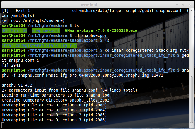 |
| The program told snaphu to unwrap the file. This is not a quick process. |
 |
| Unwrapped Phase |
And there is our final product for this tutorial!
Veci, Luis. Sentinel-1 Tookbox: Interferometry Tutorial. Array Systems Computing Inc. (2014). http://www.array.ca/
RADARSAT-2 Data and Products (c) MacDonald, Dettwiler and Associates, Ltd. (2009) - All Rights Reserved. RADARSAT is an official trademark of the Canadian Space Agency.
Tuesday, June 7, 2016
Salt Diapirism on Axel Heibger Island, Nunavut
So, what is the present objective for Elise studying radar?
![By Connormah (Based off) [CC BY-SA 3.0 (http://creativecommons.org/licenses/by-sa/3.0)], via Wikimedia Commons](https://commons.wikimedia.org/wiki/File:Axel_Heiberg_Island,_Canada.svg) |
| Axel Heiberg Island in red. |
First, what are salt diapirs? Salt, and other evapouratitic deposits, tend to be less dense than the surrounding strata. Like oil rising through water, tectonic activity can mobilize evapourite deposits, causing large mounds of salt to rise upward through the overlying rock units. The result is dome-like deformation structures surrounding the diapirs of salt.
 |
| Extent of Sverdrup Basin in the Canadian Archipelago |
Axel Heiberg Island almost exclusively part of the Sverdrup Basin. The Sverdrup Basin is a 12-15 km thick succession of strata dated from the Carboniferous up until the Eocene. The section of strata on Axel Heiberg is approximately 10 km thick; the thickest section of Mesozoic strata in the Sverdrup Basin. Approximately 100 diapirs have been found within the basin, of which 60 are exposed at surface. Three quarters of exposed diapris within the basin are located on Axel Heiberg Island. The diapirs composed of anhydrite, which is weathering to gypusum, and contain interbeds of brecciated carbonates. The basin has been subjected to numerous tectonic events, contributing to the rise of the diapirs. The basin was subject to rifting until the mid-Permian, and the basin thermally subsided between the late-Permian though the Early Jurassic. The older diapirs began their ascend during the Late Triassic, and were greatly accelerated by the onset of Arctic ocean seafloor spreading in the Cretaceous. During this time, rifting was accompanied by mafic dike swarms and flood basalt volcanism. The presence of minibasins surrounding the diapris provide evidence of regional shortening post-Late Cretaceous.
 |
| Cross-section of evaporutic diaprism on western Axel Heiberg Island. Note the younger evapourite canopy in the WABS region, where two generations of diapirism has occurred (from Harrison and Jackson, 2006). |
Post-flood volcanism and other tectonic activies were more recent folding events. The deformation structures present are not very straight forward. Most of the region is characterized by sinusoidal folds, with anticlines and synclines equally wide. These trend to the north. However, Jackson and Harrison have found a 60 km wide area of deformation where shorter folds that are out of line with the surrounding region. This area, termed a wall-and-basin structure, contains a high abundance of diapirs. They hypothesize that the wall-and-basin structure represents a canopy, where rising diapirs came together, joining to form an stratiform sheet. The style of deformation indicates a possible detachment of the strata along the salt canopy. The abundant minibasins around the wall-and-basin structure is analogous to the Gulf of Mexico, where units have also subsided over large salt canopies.
Despite being well exposed in the polar desert, the rising evapourites on Axel Heiberg Island have not been well studied. Radar analysis and remote sensing are key tools in learning more about the geological behaviour of remote sites that are difficult to field check. In measuring the rate of movement within the Axel Heiberg diapirs, we can apply this knowledge to salt diapirs in other inaccessible areas, such as politically unstable countries, and other bodies in our solar system. Salt diapirs have both economic significances, as well as geological relevance in determine the stratigraphic relationships within a basin.
This is why we are doing what we are doing, time to learn some more radar! (After convocation this week.)
Jackson, M.P.A., and Harrison, J.C., 2006, An allochthonous salt canopy on Axel Heiberg Island, Sverdrup Basin, Arctic Canada: Geology, v. 34, no. 12, p. 1045–1048, doi: 10.1130/G22798A.1.
Subscribe to:
Comments (Atom)