Sentinel-1 Toolbox Tutorials Part 2: Interferometry

Hello everyone, and here is part two of my overview of the ESA's Sentinel-1 Toolbox tutorials.  This entry is following the terrain corrections tutorial, which also uses RADARSAT-2 data.  This time we are looking over Phoenix Arizona.

Interferometry is a technique that creates a an image that does awesome cool things!  One application of interferometry explored in this tutorial is the ability to use interferograms to produce DEMs or topographic phase bands.  A similar application will be applied when I work towards my end goal project.  Remember those salt diapirs from the last post?  We will be using InSAR from different time intervals to check their height, and determine if they are moving (and if so, at what rate!)

For all intents and purposes, my M.Sc thesis is to tell the Canadian Space Agency to fire radio waves at squishy salt rocks in a polar desert, and then see how much they are oozing out of the sedimentary basin.  That is pretty great.

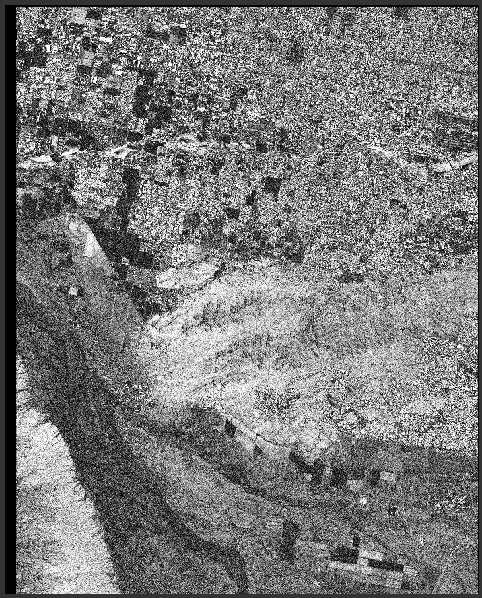
The tutorial starts us off with a set of Single Look Complex (SLC) radar images over Phoenix, Arizona.   We need to select the band we are working with, and coregister the images.

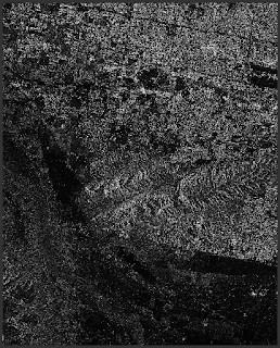One of the radar images of Phoenix, Arizona

Next, we are able to generate an interferogram from the coregistered images.  The computer does some slightly intimidating trigonometry for us, but clicking on the tools in the program is pretty easy.

Interferogram of two radar images

The space between two fringes of the same colour represents a 2pi cycle, which is half of the sensor's wavelength.  This means that the closer together the fringes, the greater the topographic variation.

In producing the interferogram, we also produced a Coherence Band which shows how similar the master and slave radar images are.

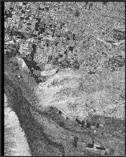Coherence Band - Dark areas have poor coherence (like vegetation, which is variable between the two images) whereas buildings have high coherence (they move less)

There is a tool we can use to "flatten" the interferogram (i.e. remove the fringes in relatively flat areas, and smooth out the topographic phases).  This tool removes the topographic phase, and effectively produces a DEM out of the interferogram.

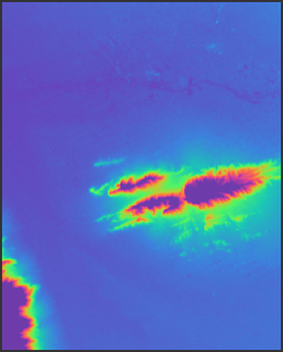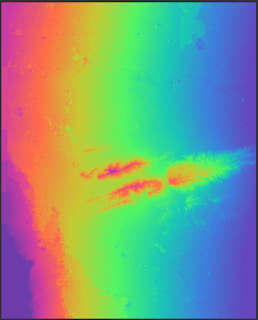
Topographic Phase Band - We produced a DEM through interferometry!

Alternatively, there are other filtering processes we can implement on the interferogram.  One way of reducing noise from temporal decorrelation, geometric decorrelation, volumetric scattering, and general processing errors through unwrapping.  Before we can unwrap the phases, we need to apply the Goldstein Phase Filtering process.  You will notice that the Goldstein filtering increases the intensity and contrast of the interferogram fringes.

Goldstein Filter on Interferogram

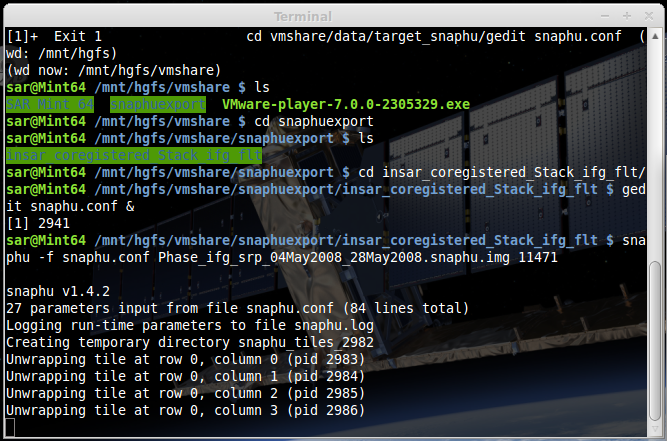
Now we are ready to unwrap, but we can't do that in Sentinel-1.  Instead, we need to export the files to SNAPHU.  SNAPHU is only available for Linux, which makes me very sad, because the command line is one of my present nemeses, along with Purolator and bagged milk.  Fortunately, the ESA tutorial provides a link to download a Linux virtual machine for Windows, through we we can run the SNAPHU program.

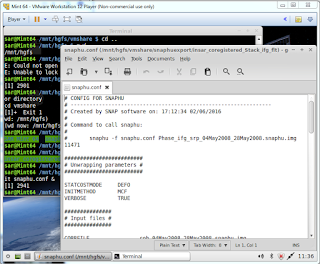Look at this silly program I had to download and figure out.  I'm Linuxing some more.

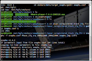The program told snaphu to unwrap the file. This is not a quick process.

Once snaphu finishes unwrapping the file (this took about two hours for me) it can be opened in SNAP or the Sentinel-1 Toolbox.  This new product needs to be unwrapped in Sentinel-1 with the wrapped file so that it may be geocoded correctly.

Unwrapped Phase

And there is our final product for this tutorial!


Veci, Luis.  Sentinel-1 Tookbox: Interferometry Tutorial.  Array Systems Computing Inc. (2014). http://www.array.ca/

RADARSAT-2 Data and Products (c) MacDonald, Dettwiler and Associates, Ltd. (2009) - All Rights Reserved. RADARSAT is an official trademark of the Canadian Space Agency.