Radarclinometry

In starting to write the SOAR-E grant proposal to attain RADARSAT-2 images over Iran, Catherine e-mailed me her 2008 paper that uses an Iranian salt diapir as a case study.  Originally the article was just so I could get the diapir coordinates, but I started to read it and found it quite interesting.

Radar topography of domes on planetary surfaces by Neish et al. (2008) introduced me to the technique of radarclinometry, which is to use radar images to produce topographic information.  By measuring variations in radar image radiance, you can find relative elevations using "shape-from-shading" techniques.  One of the largest controls on radar-backscatter values is the incidence angle at the surface.  If you imagine that a structure is homogenous, you can attribute changes in backscatter to variations in incidence angle, i.e. slope.  Once we know the slope, we can produce a topographic profile for the feature!  Neat, eh?

There are a couple of methods for this that you can use.

A one-dimensional method determines the amount of slope on a surface by measuring the brightness of lines of pixels to make a topographic profile.  This method doesn't give you any information perpendicular to your slope profile. There is a two-dimensional photoclinometry method that fits a digital topographic model to an image.  This incorporates two-dimensions, but is both slow to process and is sensitive to artifacts in the radar backscatter images.  Another method, which is employed here, uses a larger scale image of a specifically shaped feature, and adjusts the height accordingly.  This is less vulnerable to backscatter variations than the other 2-D method.

The purpose of this paper is to determine if you can use radioclinometry to measure the heights and shapes of "viscously emplaced domes", with a specific interest in studying features on Saturn's moon Titan.  The altimetry data for Titan is both sparse and poor resolution, so exploring alternative methods of gaining elevation information can have large impacts on how we study Titanean features.

What do shield volcanos and salt diapirs have in common?  They are both viscously emplaced domes! That is, they both form by the slow movement of thick, soft, deformable material, and make roughly circular shapes.  So, this study assumes a dome-shaped profile, and uses the aforementioned radarclinometry technique to measure the height profiles of viscously emplaced domes across the solar system.  The authors use an Iranian salt diapir of known elevation, and pancake domes on Venus to test their methodology before applying the technique to Ganesa Macula - a 180 km across, circular, radar-dark feature on Titan.  Ganesa Macula is suspected to have volcanic or cryovolcanic origins.

How did they do?

Well, after comparing different models, the authors found that they did a pretty good job of fitting the radarclinometry data they produced to the available topographic data available for the Iranian salt diapir. The terrestrial case study demonstrates a good proof-of-concept for this technique. In contrast, the radarclinometry profiles made for the Venusian pancake domes were consistent, but a little less than the altimetry.  Nonetheless, the heights they measured for Ganesa Macula (2.0-4.9 km) fits previous constraints, so the results are promising. They also estimate the volume of Ganesa Macula ato 30,000-40,000 km^3.  This is a significant volume, because if Ganesa Macula is made of a volcanic lava, based on Titan's heat production rates it would have to becomparable to the duration of Earth's Deccan Traps.  Perhaps Ganesa Macula is the result of a rare event, which would explain why it is such a unique feature on Titan.

I expect that next time I write I'll have fixed the registration issue with my radar images.  I look forward to showing you my PALSAR acquisitions!

Cheers!

From one desert to another

With the intent of returning to the image misregistration issue once I'm back from Québec, I've been switching gears into proposal-writing mode.

Catherine and I have discussed the possibility of extending our work to compare and contrast our Axel Heiberg Island diapirs to those in the Zagros Mountains, Iran. I have frequently referred to Axel Heiberg Island as "having the second highest concentration of salt diapirs in the world".  Well, Iran has the first-highest concentration of salt diapirs in the world.  These two sites would be interesting to compare for multiple reasons.

1. They are both desert environments, meaning that radar signals are less likely to be affected by soil moisture or obstructed by vegetation.
2. They are different types of desert environment.  Axel Heiberg Island is a polar desert, where cryoturbation is the predominant weathering mechanism.  Iran is a hot desert, with aeolian processes, gravity-driven mass movements, and periodic flashflooding as predominant weathering mechanisms. Different erosion mechanisms may lend to observable differences in surface roughness of the diapirs and surrounding rock units.
3. The diapirs have different compositions.  The salts on Axel Heiberg Island are predominantly anhydrite (CaSO4) weathering to gypsum (CaSO4 * H2O), whereas the salts in Iran are more classic halite rock salt (NaCl). Both salts are soft and soluble, but have different crystal structures which may lend to different radar responses and erosion patterns.

To initiate this change of pace, Catherine has asked me to write a draft proposal for the CSA's SOAR-E program.  RADARSAT-2 images aren't free, so this program let's us pitch our wonderful science ideas to the CSA and request access to their data.  I have not written a proposal before, so this is a slightly intimidating, but beneficial, experience.

Unfortunately there do not appear to be any PALSAR-1 Quad-Pol acquisitions over Iran, so we will not be able perform the same comparison between C-band and L-band for the Iranian diapirs.

PALSAR Hiccups

Hi hi~

Last post, I mentioned that we had acquired (or at least were in the process of acquiring!) quad-polarized images from the Phase Array L-Band Synthetic Aperture Radar (PALSAR) on Japan's Advanced Land Observing Satellite (ALOS).  The images have been downloaded, and processing near completed!  I've made multilooked and terrain corrected HH Intensity images and CPR images.

However, there is a bit of a problem.

If you look closely at some of the acquisitions, you can see that there is some kind of image artifact running East-West through some of them.  This artifact does not exist in the raw level 1.1 images, and it only seems to appear after the terrain correction step.

I consulted Mike, an experienced post-doc in the Neish lab research group, about the artifacts and he suggested I start troubleshooting by looking at the DEM I'm using for terrain correction.  This is the also same DEM that I've been using for the RADARSAT-2 images, and I've subsequently noticed the same error in these images as well.  Despite the DEM being a mosiac, there does not appear to be any visible seam in the image which could have caused the trouble.  Catherine thinks there is a misregistration issue, which could be manually resolved if other troubleshooting methods fail.  We might also try terrain correction with a different DEM.

I'm hesitant to report specific CPR data analysis until after this is fixed, but we can make some preliminary observations from what we have.

Salty surfaces are seem to be a little bit rougher in PALSAR's L-band radar than in RADARSAT-2's C-band radar, with salt domes having average CPR values of 0.45 (average CPR of domes - taking the average of the mean CPR for measured salt domes) or 0.51 (average pixel value for all measured salt domes).  In comparison, the RADARSAT-2 has average CPR values of ~0.40 (for both average of domes, and average per pixel).  The difference between CPRs of 0.4-0.5 might not be too significant, but we can at least see that the diapirs are appearing rough over a range of scales.

The average CPR for remobilized salt deposits appears significantly rougher in L-band than C-band. This, however, appears to be attributed to two anomalous deposits. Of 14 measured deposits measured in L-band, two appear to have average CPR > 1, whereas the remaining deposits have a diverse range of averages from 0.14-0.56.  In comparison, salt deposits in C-band show far more constrained average values between 0.23-0.38, with the mean of average deposits (0.28) being closer to mean pixel value (0.26).  This might mean that a few of the deposit areas are not smooth sands as previously interpreted, but are actually filled with cobble-sized clasts that area being noticed at the longer L-band wavelength and not the shorter C-band.  It would be interesting to field check these different deposits to validate this hypothesis.

I'm out of town next week (wooo!  I'm visiting Québec City for the Winter Carnival!) but we will return to this problem once I'm back.

New Year and Fresh Starts

Hello everyone, and Happy New Year!

I'm back at Western after a wonderful winter break with my family in Vancouver.

Some general house-keeping:

In my first week back, I've been doing some general "house keeping" with my data.  I'm getting myself organized by deleting duplicate and unwanted files from awry processing.  I think it is a common problem: if you are trying a new tool in ArcGIS, are processing a new dataset, or input the wrong variable, you get erroneous files. I know that at least for me, these mistakes can sometimes get ignored as I'm too focused on "getting it right", and these can clutter up folders with the good data. I'm getting rid of these, and also making sure everything is labeled so data is easy to find and folders are easy to navigate.

On a tangent, it is also important to make sure you have good "metadata" or data about your data. For the RADARSAT-2 images I'm working with, I make sure to include notes about the number of looks in the azimuth and range directions when doing multilook processing. This lets me know how smoothed over my images are.  The numbers of looks are different depending on the end products. For example, CPR images tend to be very noisy, so I use more looks for CPR images than when I'm performing a Pauli Decomposition. It is important that I, and anyone else who may need to look at my files, know what I did, so I'm working on making a key that explains my data.

At AGU in December, one of the workshops I attended during the Student & Early Career Scientists Conference focused entirely on  "Improving Your Science Through Better Data Management", and I learned a few tricks that I'm starting to implement. Not that you need any convincing, but here is a cute cartoon they shared that further emphasizes why data management is important, especially when you might need to share data with other scientists.

Moving forward - Acquiring PALSAR data:

My data management is being done now to prepare for the incoming of new data!  Yay, new data!

I have recently put in a request to the Alaska Satellite Facility to get data from the Japan Aeronautics Exploration Agency's Advanced Land Observing Salilite (ALOS).  ALOS had an L-band radar, called PALSAR. Like RADARSAT-2, PALSAR also has fully polarimetric capabilities. The two radars have different wavelengths. RADARSAT-2 is a C-band radar, with a wavelength of 5.5 cm, while PALSAR's L-band has a wavelength of 23.6 cm. We can use both datasets together to explore the surface roughness at different scales.  For example, surfaces that look rough in C-band radar may appear rough in L-band radar, and vice versa.  Comparing apparent roughness at different scales from the two different radar instruments can help us constrain the scale of surface roughness of the salt diapirs on Axel Heigberg Island.

I'm a little disappointed that there isn't very much PALSAR quad-pol coverage of our study site in Expedition Fiord, but it does look like at least a couple prominent diapirs are covered, so we will focus on those.

Batch Processing:

It was brought to my attention that I can really speed up radar data processing by implementing "batch processing" i.e., doing multiple images at once.  This will be really useful when the PALSAR data comes in, so I'm testing it out with my RADARSAT-2 images in SNAP.  So far I have not succeeded, but I've only just started playing around and troubleshooting.

Maybe some basic programming will help with that, speaking of which...

Developing computer skills:

One of my colleagues here at Western, Denis Vida, has put together an informal, non-credit Python Immersion course/workshop. My programming abilities are wanting, and if you remember from before I can barely navigate a command line, (barely, but I can!😊) My previous Python experience is limited to completing the Codecademy online course, most of which needs much refreshing. Fortunately, Denis has referred us to a free, online tutorial on computer programming through Udacity that I am going through to get up to speed. Looking through the e-mailing list for the workshop, it looks like I will be in good company with most of my labmates also attending.

2016 American Geophyical Union Fall Meeting

Hi hi~

I am very grateful to have had the opportunity to attend the American Geophysical Union Fall Meeting in December.  It was a great experience to meet new people, reconnect with colleagues,attend career development workshops, learn about the cutting edge of geology, geophysics, and planetary science, and have the opportunity to present my own research.

This post may seem lengthy, but I'm also partially writing it as a means to refresh myself with all the events from the conference. The week went past like a whirlwind, and there were a lot of interesting topics I'd like to follow up on.  I hope you're interested, too!

View of the Moscone South building (Poster Hall) from Moscone West (Oral Sessions)

Highlights

Student & Early Career Scientists Conference

I arrived a day early to attend the Student & Early Career Scientist Conference - a daylong series of career development workshops. Only a few weeks prior I had made an offhand comment to my labmate Gavin that I wished there were courses we could take on data management, and making scientific figures. To my delight, this event offered both! Hour long talks included, "Making Figures Talk: Data Visualization for Scientists" and "Improving Your Science Through Better Data Management: Tips and Techniques".  The notes from the data visualization workshop are available online if you're interested. A couple tips I plan on trying are using white instead of black lines on bar graphs to make them sharper, and using partial transparency on scatter plots to see overlapping points. We were also warned that the "rainbow" colour scale, frequently used for raster datasets, has a couple sharp steps that can make it seem like there is a bigger change than their really is. This is something to keep in mind, because we use the rainbow scale for our CPR images.

Exhibitor Hall

Exhibitor's Hall, immediately upon opening

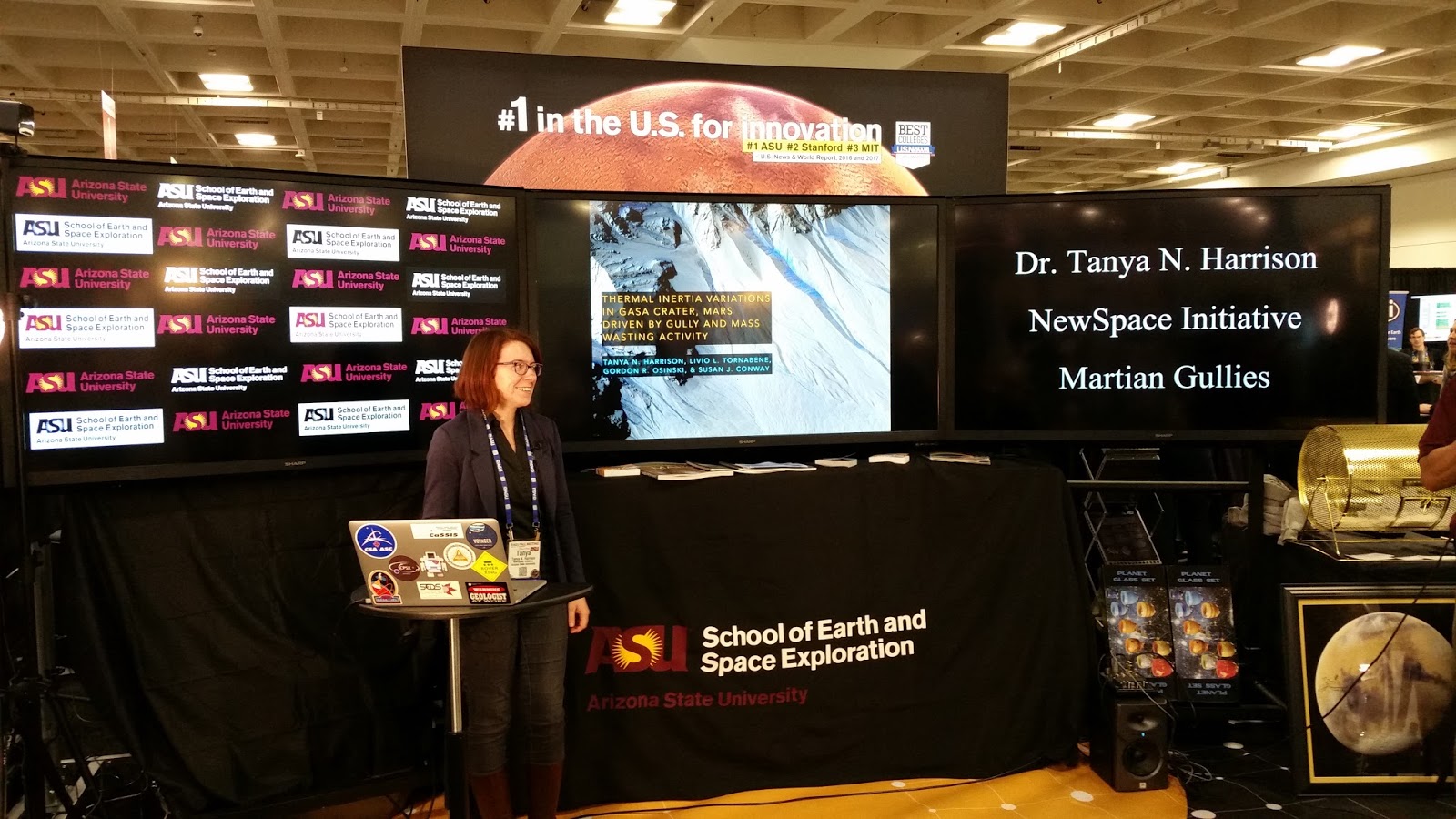
Okay, aside from the ridiculous amounts of swag collected (many new posters are now decorating my apartment) there were a lot of interesting things going on in the Exhibit Hall.  The Google booth hosted many short talks on using remote sensing to monitor and study global environmental issues. Western alumni, Tanya Harrison, had a featured talk on Martian gullies at Arizona State University's booth.

Western alumni, Tanya Harrison, gives a talk on Martian Gullies

I also learned that many Asian institutions are running hiring initiatives to attract foreign early career scientists for new faculty positions.  If you are a post-doc interested in working in Asia, this is your time to shine.

Poster Hall

Tim Haltigin from the Canadian Space Agency presented a well-designed, highly popular poster on the 2016 CanMars mission.  CanMars was a highly successful, collaborative analogue Mars sample return mission that ran mission control operations here at Western last November. I had the pleasure of taking part in the mission as a member of the GIS & Mapping team, and am thoroughly grateful for the opportunity.

Maria's poster and my talk complimented each other really well.  She presented the results from her internship with Dr. Neish over the summer, using thermal infrared spectroscopy to identify and map anhydrite salt exposures on Axel Heiberg Island, NU.  I presented results in which I extracted the zonal statistics for CPR values in the areas she mapped as salt. Unfortunately, her poster presentation was during the time slot of my oral session, so I wasn't able to visit her during poster-time, but I did have the privilege to talk with her about it before and after.

Really cool radar stuff: I roamed through a few really interesting poster sessions that employed polarimetric radar for planetary atmospheres and meteorological studies. In the back of my mind, I was vaguely aware that this was a thing people do, but hadn't previously thought about how it works. Many studies explored the  using different bands of polarimetric radar to estimate precipitation and storm intensity, which is important in risk assessment in coastal nations like Korea (Gu et al. 2016; Lim et al. 2016). One of the studies measured the distribution of raindrop size, which can then be correlated with the storm severity for hazard prevention. Another study uses C and S band radar for distinguishing size of hail particles, which is important in central Europe where hail can be the size of tennis balls (Schmidt et al. 2016).

Not radar, but another session focused on using passive polarimetry as a tool to study planetary bodies, including spaceweathering on the moon (Kim et al. 2016), the surface texture of Europa (Nelson et al. 2016), and even the composition of organics in meteorites (Kobayashi et al. 2016)

Oral Sessions

One of my favourite oral sessions entailed a group of prominent Mars researchers discussing Mars's past as either "cold and dry" or "warm and wet".  I didn't realize that the "cold dry Mars" theory had much footing, but field analogues from Dry Valleys, Antarctica shows that even in very cold dry places there is significant seasonal melting that can form erosional features (Head 2016). Robin Woodsward similarly suggests that early Mars may have been more Titan-like, with a cold, dry climate and episodic melting that can explain fluvial features (Wordswarth 2016).  I had the pleasure of meeting some of the presenters after this session and discussed current advancements in planetary science.

My talk was also quite successful!  Despite being in the last session of the final day, there was a reasonable turn out. I met Dr. Gerald Patterson and Dr. Lynn Carter before the session, and they were both positive and asked insightful questions after my talk. Another gentleman approached me afterwards, asking if we have used any Sentinel-1 data for our student.  We have not, but I mentioned that we are about to request PALSAR data.  The other talks in this session were really interesting, too.  One gentleman from Arceibo gave an overview of how Arecibo is used for planetary exploration (Taylor 2016).  Dr. Carter gave a talk about how they have constructed giant vats of ice and sediments at the Goddard Flight Center to try and simulate data from SHARAD, the shallow ground penetrating radar orbiting Mars (Carter et al. 2016).

Social Events

The NASA hosted Planetary Science division Townhall.  I met Jim Green, and asked about the current relationship and collaborations between NASA and the CSA. Bethany Ehlmann from Caltech was also a speaker at this session. I worked with her during our Arctic field season last summer, and it was great to see her again.

Bethany's career advice for students and early career scientists,
1. Don't give up on your rejected proposals
2. Papers. Papers, papers, papers. Grad students should focus on writing good papers.

Panelists at the NASA Planetary Science Division Townhall meeting

I also attended the Planetary Science meeting/reception, and the earth and planetary surface processes reception. Both events were great for networking. I reconnected with colleagues from LPI, and met sedimentologists from the University of Bristol who introduced me to a few prominent Martian surface scientists.

San Francisco

Of course, I also took time to explore San Francisco!  I had never been to the city before, and was able to have the chance to visit Chinatown, Fisherman's Wharf, and Pier 39.One of my favourite parts of traveling is trying local food, so I'm happy that I was able to eat some dim sum, sourdough bread, and Ghirardelli chocolate.

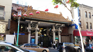
Fancy bank in Chinatown

View of Alcatraz prison from Fisherman's Wharf

Golden Gate Bridge as seen from Fisherman's Wharf

SOURDOUGH BREAD FACTORY! YUM!

Overall, I highly recommend the American Geophysical Union Fall Meetings. I had a great time, learned lots, and met a lot of incredible people.  Cheers!

The 7th Canadian Space Exploration Workshop

A fortnight ago, I had the pleasure of attending the 7th Canadian Space Exploration Worksop (CSEW).  The CSEW was a two day workshop hosted by the Canadian Space Agency in Montreal.  The purpose of this meeting is for scientists involved in Canadian space and planetary science to convene and discuss what science objectives should be prioritized over the next decade.  The Canadian Space Agency then takes these priorities into strong consideration when determining funding allocations going forward.  The stronger a grant proposal is inline with these objectives, the more likely it is to be selected.  The last meeting of this nature was seven years ago in 2009.  You can read theobjectives outlined at the 2009 6th CSEW here. This meeting is therefore vital, not only for networking and becoming up-to-date with recent research in space science, but also in guiding decisions that will affect our future career paths as planetary scientists working in Canada.

CSEW 2016 was held in the Marriott hotel.  The Planetary Exploration
topical sessions were held on the 36th floor, with this lovely view.

Not only research scientists were present.  Many of attendees comprised doctors, engineers, and representatives from industry and governmental organizations. 

Attendees divided themselves into nine topical teams based on their interests in Planetary Exploration, Space Astronomy, or Space Health and Life Sciences:

Planetary Exploration

1. Astrobiology
2. Planetary Atmospheres
3. Planetary Geology, Geophysics & Prospecting
4. Planetary Space Environment
    

Space Astronomy

5. Cosmology, Dark Energy, and Cosmic Microwave Background
6. Origins and Evolution of Galaxies, Stars and Planets
7. High Energy Astrophysics (HEA)

Space Health and Life Sciences

8. Multidisciplinary Approach to Health Risk Mitigation in Space
9. Space Radiation Risk to Humans: Identification, Characterization & Mitigation

This year's Canadian Space Exploration Workshop had a special focus on the Space Health and Life Sciences topical teams, but each of the nine disciplines updated their science priorities.

It should come as no surprise that I attended the 3rd topical team, on Planetary Geology, Geophysics & Prospecting.  It is worth noting that attendees were not restricted to any one section.  Many people bounced amongst the geology, astrobiology, and atmospheres rooms. 

The Planetary Geology, Geophysics & Prospecting topical team was led by Western's own Dr. Gordon Osinski. [twitter link].  In fact, the University of Western Ontario and the Centre for Planetary Science and Exploration had a strong presence at the meeting, with myself, Dr. Livio Tornabene, Patrick Hill, Etienne Godin, alumni Haley Sapers and a student from the department of Physics and Astronomy present.  Myself and Patrick filled the documentarian roles at Dr. Osinski's sessions, keeping notes following our changes in science priorities and the justifications for our decisions.  You may notice that the term "prospecting" is in the name of this topical session.  Indeed, Asteroid Mining has been newly listed amongst Canadian Space Science Priorities!  The future is coming.

Our discussions were quite intensive!  We began the session with 18 potential objectives drafted.  Our target was 5-6, so this may have been overboard!  Amongst these objectives were planet-specific priorities, like determining if there is active volcanism on Venus, and exploring geological and geochronologic record preserved in Mercurian crust.  This approach was new, as neither Venus nor Mercury, received any specific priorities in the 2009 CSEW.  However, this approach did not last.  We soon, somehow, cut ourselves down to only three objectives, which were far too broad in focus!  Finally, an equilibrium was established, and we are pleased to have shared six ideas for new objectives for submission. 

These objectives are drafts, open to further input, and will be subject to much refinement, but have been proposed to be along the following lines:

Objective 1:  Document the geological record and the processes that have shaped the surfaces of the terrestrial planets and their moons, asteroids (e.g. impacts and volcanism).

Objective 2:  Determine the interior structure and properties of the terrestrial planets and their moons, and asteroids.

Objective 3:  Determine the resource potential of the Moon, Mars, and asteroids

Objective 4:  Surface modification processes on airless bodies (space weathering, regolith processes, micrometeroites, solar wind)

Objective 5:  Understand the origin and distribution of volatiles (e.g. water ice) on the terrestrial planets and their moons, asteroids, and comets)

Objective 6:  Impact threat and hazards

One of the emphases explored by Objective 1 is the role of planetary analogue studies.  Analogue studies involve using rocks or climate systems on Earth to better understand similar features on other planetary bodies, and are something Canada excels at.  Scientists from around the world come to Canada to use our country's diverse range of climates, rock types, tectonic systems, and environments.  It has been put forward for CSA to instate a small grants program for terrestrial field analogue studies, and this was met with a positive response.

A second priority listed is for Canada to contribute a synthetic aperture radar contribution to an upcoming Mars orbiter mission.  Radar systems, like my favourite RADARSAT-2 that I use for my thesis, are also something Canada excels at.  The Canadian Space Agency works in conjunction Vancouver based MacDonald, Dettwiler and Associates Ltd (MDA corporation) to develop these orbiters.  Synthetic aperture radar is missing from the Mars orbital datasets, and a Canadian contribution would be most welcome to fill this niche.  Not only is radar is excellent for characterizing the roughness of surfaces, but polarimetric radar is also extremely useful in identifying water ice -something that has been a target of multiple Mars exploration missions, like the Phoenix lander.

All in all, I think the meeting was quite successful!  And not just because I'm biased towards radar and field analogue studies. 😊

Fortunately if you were unable to attend this year, you may not need to wait another seven years for the next workshop.  One of the unanimous sentiments shared by scientists at the meeting was that we felt like there was too much to discuss and catch up on, in such a short time.  The Canadian Space Agency hopes to run CSEWs at more regular intervals going forward, and I hope to see you there!

Rocky roads and smooth sailing

Hello, hello.

So, as previously mentioned, the hypothesis of this project is that solubility of salt diapirs will lend them into eroding into different patterns than other sedimentary strata.  An outcome of this are rillenkaren features; grooved furrows that arise on the surfaces of inclined diapirs [1].  Because of the erosion patterns of diapirs, we expect to correlate diapirs with rougher radar signatures, and are testing this hypothesis with our new RADARSAT-2 images.  You can see our freshly terrain corrected and processed CPR images in this previous post.

Our goal for this part of the project is to compare and contrast the mean and distribution RADARSAT-2 CPR values in the salt exposures against the surrounding rock type.  To do this, we have overlain shapefiles made by Maria.  She used ASTER TIR to isolate regions with strong anhydrite signatures.  She also made shapefiles outlining the salt diapirs as mapped by Harrison and Jackson (2014) [2].  I took the averages of CPR in these areas, and found something concerning:

The averages of the salt are pretty similar to the surrounding rock.

Figure 1: All rocks CPR distribution (histogram slightly stretched).  Average CPR: 0.32

Figure 2:  All salt (Mapped by Maria) CPR distribution.  Average CPR: 0.40

I mean, a ~0.08 difference isn't necessarily insignificant, but the individual rock units range in average CPR from 0.25 in areas with the Invincible Point Member (silty shale) and Wolf Tongue (fine-grained sandstone-siltstone) and up to 0.43 in the Awingak Formation (quartz sandstone with interbedded shale).  That is odd.  Just look at our images and see that the salt diapirs have higher CPR values than the surrounding rock. (Well, except for those anomalously high-CPR areas in the south... We'll investigate those soon.)

Yup, looks rough, as expected.

But, alas.  When looking at some of our salt signatures in more detail, we can see that there are some that are very radar-smooth!

Wait, what are you doing here?

These low CPR areas all seem to be located in low-elevation valley areas, or slopes!  Interesting! I double checked with the ASTER TIR, and confirmed that these areas do, in fact, correspond with areas of strong anhydrite signatures.  I think this means that we have anhydrite sediments eroding out of the diapir (and concordant salt exposures), and are remobilizing and depositing in lowland areas.  Water erodes rock.  Gravity makes things fall down.  Simple explanation.

Supporting this hypothesis: one particularly interesting spot has high CPR at the higher elevation, and low CPR at the lower elevation.  In the ASTER TIR, the signature is stronger at the top than the bottom.  One point for the remobilization hypothesis!

Part of outline salt region that is brighter (red) in CPR corresponds with a higher elevation, as well as as a stronger TIR signature than the lower, darker area.

This was actually something we considered over the summer, before we processed any of the RADARSAT-2 images.  Conveniently, we had already asked Maria to make subsets of her ASTER TIR salt map:  One maps areas of suspected remobilized sediment, and another shows areas corresponding to suspected domes/diapirs.  Now, these were visually assessed, and there is room for error in the polygon outlines, but the shapefile provides a solid starting point for performing a more in depth, targeted analysis.  If we run the same procedure on these subset shapefiles, we get the following:

CPR histogram for salt signatures visually classified as "remobilized" sediment deposits.  Mean: 0.26.

CPR histogram for salt signatures classified as "diapirs" or "domes" through visual mapping and comparisons with previous field mapping [2].  Mean: 0.43

Huzzah!  These results make much more sense!  We can clearly see that the eroded anhydrite sediments are being redeposited in smooth areas, while the diapirs are eroding into rougher surfaces, as hypothesized!

One note for concern: the mean value for diapir CPR, while certainly higher than mean CPR for other rocks, is still comparable to some of the clastic rock units.  These are the Awingak and the Heiberg Formations.  As previously mentioned, the Awingak Formation consists of quartz-sandstones.  In contrast, the Heiberg Formation comprises interbedded sandstone, siltstone, and shale (interpreted as a deltaic-sandstone facies) [2].  These areas might be (are likely) the radar-bright regions in the southern portion of our CPR mapping, and will be investigated in the near future.

Using areas mapped by Harrison and Jackson [2] provide different results as well.  Taking the CPR from areas strictly mapped as Otto Fiord Formation (our evaporites) we get a mean of 0.37.  But, if you map CPR of areas with Otto Fiord Formation with carbonates or breccia, you get considerably higher values of 0.53 and 0.72!  Wow!  I have not yet explored where on the map these exposures are located, or if they correspond with some of Maria's shapefiles, but these results are certainly worth investigating further.

Note, that average values reported for rock formations are taken as an average of the averages of each of the mapped areas.  In contrast, the averages and distributions for Maria's shape files are reported as average/pixel.  I also took the averages/average area for Maria's areas to compare, and there is a <0.0225 discrepancy for each subset of salt regions.  While plausibly minor, there some room for discrepancy in the mapped rock units.

Two variables which may be influencing CPR returns are RADARSAT-2 beam modes, and localized slope (affecting the incidence angle of the radar beam).

The beam modes used for our images include FQ19W, FQ20W, FQ21, and FQ21W.  "FQ" means that the images were taken with Wide Fine Quad Polarization, providing us with larger target areas and finer resolutions than standard images, as well as full polarization images (HH+VV+HV+VH). These correspond with near incident angle ranges from 37.7°-40.2°, and far incidence angles from 40.4°-42.1° [3].  Slopes will also affect local incidence angle, and thus the amount of radar return.  Slopes facing the incident beam will reflect stronger signals than those reflecting away.  

Well, that was more than your daily dose of diapirs and domes and salts (oh my)!

Happy mapping!

P.S. I presently don't know to make better histograms from ArcMap, than those I've extracted from the symbology tab.  Looking for any advice on how to improve my data representation, or how to export the data for use in other programs!

[1] Stenson, R.E., and Ford, D.C. 1993. Rillenkarren on gypsum in Nova Scotia. Geographie physique et 
               Quaternaire, 47: 239–243.

[2] Harrison and Jackson (2014) Exposed evaporite diapirs and minibasins above a canopy in central Sverdrup 

               Basin, Axel Heiberg Island, Arctic Canada. Basin Research 26, 567–596, doi: 10.1111/bre.12037

[3] MacDonald, Dettwiler and Associates Ltd. 2016. RADARSAT-2 product description. MacDonald, Dettwiler and Associates Ltd. RN-SP-52-1238 1(13), Richmond, B.C. Available from  http://mdacorporation.com/docs/default-source/technical-documents/geospatial-services/52- 1238_rs2_product_description.pdf?sfvrsn=10 [accessed 28 October 2016].

RADARSAT-2 Data and Products (c) MacDonald, Dettwiler and Associates, Ltd. (2016) - All Rights Reserved. RADARSAT is an official trademark of the Canadian Space Agency.