Rocky roads and smooth sailing

Hello, hello.

So, as previously mentioned, the hypothesis of this project is that solubility of salt diapirs will lend them into eroding into different patterns than other sedimentary strata.  An outcome of this are rillenkaren features; grooved furrows that arise on the surfaces of inclined diapirs [1].  Because of the erosion patterns of diapirs, we expect to correlate diapirs with rougher radar signatures, and are testing this hypothesis with our new RADARSAT-2 images.  You can see our freshly terrain corrected and processed CPR images in this previous post.

Our goal for this part of the project is to compare and contrast the mean and distribution RADARSAT-2 CPR values in the salt exposures against the surrounding rock type.  To do this, we have overlain shapefiles made by Maria.  She used ASTER TIR to isolate regions with strong anhydrite signatures.  She also made shapefiles outlining the salt diapirs as mapped by Harrison and Jackson (2014) [2].  I took the averages of CPR in these areas, and found something concerning:

The averages of the salt are pretty similar to the surrounding rock.

Figure 1: All rocks CPR distribution (histogram slightly stretched).  Average CPR: 0.32

Figure 2:  All salt (Mapped by Maria) CPR distribution.  Average CPR: 0.40

I mean, a ~0.08 difference isn't necessarily insignificant, but the individual rock units range in average CPR from 0.25 in areas with the Invincible Point Member (silty shale) and Wolf Tongue (fine-grained sandstone-siltstone) and up to 0.43 in the Awingak Formation (quartz sandstone with interbedded shale).  That is odd.  Just look at our images and see that the salt diapirs have higher CPR values than the surrounding rock. (Well, except for those anomalously high-CPR areas in the south... We'll investigate those soon.)

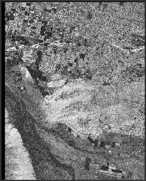
Yup, looks rough, as expected.

But, alas.  When looking at some of our salt signatures in more detail, we can see that there are some that are very radar-smooth!

Wait, what are you doing here?

These low CPR areas all seem to be located in low-elevation valley areas, or slopes!  Interesting! I double checked with the ASTER TIR, and confirmed that these areas do, in fact, correspond with areas of strong anhydrite signatures.  I think this means that we have anhydrite sediments eroding out of the diapir (and concordant salt exposures), and are remobilizing and depositing in lowland areas.  Water erodes rock.  Gravity makes things fall down.  Simple explanation.

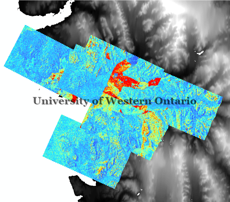
Supporting this hypothesis: one particularly interesting spot has high CPR at the higher elevation, and low CPR at the lower elevation.  In the ASTER TIR, the signature is stronger at the top than the bottom.  One point for the remobilization hypothesis!

Part of outline salt region that is brighter (red) in CPR corresponds with a higher elevation, as well as as a stronger TIR signature than the lower, darker area.

This was actually something we considered over the summer, before we processed any of the RADARSAT-2 images.  Conveniently, we had already asked Maria to make subsets of her ASTER TIR salt map:  One maps areas of suspected remobilized sediment, and another shows areas corresponding to suspected domes/diapirs.  Now, these were visually assessed, and there is room for error in the polygon outlines, but the shapefile provides a solid starting point for performing a more in depth, targeted analysis.  If we run the same procedure on these subset shapefiles, we get the following:

CPR histogram for salt signatures visually classified as "remobilized" sediment deposits.  Mean: 0.26.

CPR histogram for salt signatures classified as "diapirs" or "domes" through visual mapping and comparisons with previous field mapping [2].  Mean: 0.43

Huzzah!  These results make much more sense!  We can clearly see that the eroded anhydrite sediments are being redeposited in smooth areas, while the diapirs are eroding into rougher surfaces, as hypothesized!

One note for concern: the mean value for diapir CPR, while certainly higher than mean CPR for other rocks, is still comparable to some of the clastic rock units.  These are the Awingak and the Heiberg Formations.  As previously mentioned, the Awingak Formation consists of quartz-sandstones.  In contrast, the Heiberg Formation comprises interbedded sandstone, siltstone, and shale (interpreted as a deltaic-sandstone facies) [2].  These areas might be (are likely) the radar-bright regions in the southern portion of our CPR mapping, and will be investigated in the near future.

Using areas mapped by Harrison and Jackson [2] provide different results as well.  Taking the CPR from areas strictly mapped as Otto Fiord Formation (our evaporites) we get a mean of 0.37.  But, if you map CPR of areas with Otto Fiord Formation with carbonates or breccia, you get considerably higher values of 0.53 and 0.72!  Wow!  I have not yet explored where on the map these exposures are located, or if they correspond with some of Maria's shapefiles, but these results are certainly worth investigating further.

Note, that average values reported for rock formations are taken as an average of the averages of each of the mapped areas.  In contrast, the averages and distributions for Maria's shape files are reported as average/pixel.  I also took the averages/average area for Maria's areas to compare, and there is a <0.0225 discrepancy for each subset of salt regions.  While plausibly minor, there some room for discrepancy in the mapped rock units.

Two variables which may be influencing CPR returns are RADARSAT-2 beam modes, and localized slope (affecting the incidence angle of the radar beam).

The beam modes used for our images include FQ19W, FQ20W, FQ21, and FQ21W.  "FQ" means that the images were taken with Wide Fine Quad Polarization, providing us with larger target areas and finer resolutions than standard images, as well as full polarization images (HH+VV+HV+VH). These correspond with near incident angle ranges from 37.7°-40.2°, and far incidence angles from 40.4°-42.1° [3].  Slopes will also affect local incidence angle, and thus the amount of radar return.  Slopes facing the incident beam will reflect stronger signals than those reflecting away.  

Well, that was more than your daily dose of diapirs and domes and salts (oh my)!

Happy mapping!

P.S. I presently don't know to make better histograms from ArcMap, than those I've extracted from the symbology tab.  Looking for any advice on how to improve my data representation, or how to export the data for use in other programs!

[1] Stenson, R.E., and Ford, D.C. 1993. Rillenkarren on gypsum in Nova Scotia. Geographie physique et 
               Quaternaire, 47: 239–243.

[2] Harrison and Jackson (2014) Exposed evaporite diapirs and minibasins above a canopy in central Sverdrup 

               Basin, Axel Heiberg Island, Arctic Canada. Basin Research 26, 567–596, doi: 10.1111/bre.12037

[3] MacDonald, Dettwiler and Associates Ltd. 2016. RADARSAT-2 product description. MacDonald, Dettwiler and Associates Ltd. RN-SP-52-1238 1(13), Richmond, B.C. Available from  http://mdacorporation.com/docs/default-source/technical-documents/geospatial-services/52- 1238_rs2_product_description.pdf?sfvrsn=10 [accessed 28 October 2016].

RADARSAT-2 Data and Products (c) MacDonald, Dettwiler and Associates, Ltd. (2016) - All Rights Reserved. RADARSAT is an official trademark of the Canadian Space Agency.

Pauli Decomposition

Hello again, and welcome to another week of Arctic Resolution.

Last post, we explored the new 2016 RADARSAT-2 Acquisitions we obtained over the Expedition Fiord region of Axel Heiberg Island, Nunavut.  I showed you derived Circular Polarization Ratio (CPR) images of our study area.  This week is similar.  Since producing the CPR maps, I have compiled a set of Pauli decomposition images for our site.

What is a Pauli decomposition?  Pauli decompositions are used to show scattering mechanisms affecting the roughness of a surface.  In this way, they are very similar to CPR images; albeit more qualitatively interpreted.  CPR is calculated as a single integer, in which surfaces can be categories as smooth (CPR <<1), moderately rough (CPR ~0.5-1), or blocky (CPR >1).

In contrast, Pauli decompositions are more interpretive.  They are represented as RGB composite images, with the colour red being derived from the HH and VV bands: |HH-VV|^2; green from the HV band: |2HV|^2; blue also from HH and VV: |HH+VV|^2.  Recall that we are using quad-polarimetric radar, which takes advantage of RADARSAT-2's capability of transmitting and receiving horizontal and vertical signals.

What does this ultimately mean?  Areas of the images that feature more red highlight areas of double-bounce scattering, like blocky surfaces or ice.  Green areas show multiple-bounce scattering, which are rougher surfaces.  Blue shows single-bounce radar, which will indicate smoother surfaces.  Of course, these images are composites, so very few places will show solely one colour, with lots of purples and yellows indicating multiple types of radar return.  This fact exemplifies that Pauli decompositions are qualitatively interpreted; they look pretty, but caution is advised when characterizing surfaces.

Like the last post, the images are terrain corrected in SNAP, and uploaded into ArcGIS.  Unlike the previous CPR images, we did not use PolSARPro at any step during the processing.  All of the processing was performed in SNAP, as follows:

• Radiometric calibration
• Multilooking (we went with 4 azimuth looks this time, instead of 6)
• Pauli decomposition
• Terrain correction (Range-Doppler)
• Export to ArcGIS

For some reason, though, some of our images look silly!  Instead of looking like a regular Pauli decomposition, a few took on very bright pinks, blues, and greens.

Pauli decomposition produces an RGB composite image, with purple, yellowish and greenish colours most common.  The bright pink and aqua is the result of a stretching issue.

I was able to fix this problem by setting NoData values to 0 in each of the images, which removed pixels that were offsetting the histograms used in stretching the images.  I haven't stretched the images on the same scale, yet, but you can see they look much better.

Pauli decomposition of 2016 RADARSAT-2 acquisitions, masking out areas of 0 elevation (i.e., water).  Images are not mosaiced or stretched on the same scale.  

Pauli decomposition of 2016 RADARSAT-2 acquisitions, including water.  Images are not mosaiced or stretched on the same scale.

Comparing differences between the water-inclusive and water-exclusive compliations, as well as colour tone discrepancies among images within the same compilations, shows the importance that image stretching plays when we interpret these images.  Remember, since Pauli decompositions are qualitatively interpreted, consistency is very important.

A preliminary assessment, though, shows that our large salt dome is yellow, which suggests that this area is rough, with a combination of double-bounce scattering (red band) and multiple bounce scattering (green band).  This is consistent with the high CPR signature seen previously.

RADARSAT-2 Data and Products (c) MacDonald, Dettwiler and Associates, Ltd. (2016) - All Rights Reserved. RADARSAT is an official trademark of the Canadian Space Agency.

HiRISE Images!

And now for something completely different.

This past month I've been working on another project outside of my Arctic radar thesis work: my first planetary mission experience!  I've had the pleasure to be involved a 2-week imaging campaign for HiRISE - the highest resolution imager in Mars orbit.  Many of you have heard me mention that I've been working on HiRISE lately, so here is some explanation of what that means.

HiRISE (High Resolution Imaging Science Experiment) is an instrument on the Mars Reconaissance Orbiter (MRO), which has been in orbit since 2006.  As the MRO orbits Mars, HiRISE takes very high resolution images (~25-30cm/pixel) of the surface of Mars.  These images are used for geological mapping, interpreting surface features, and even exploring both the science and safety of candidate landing sites for future Mars missions.

Artist rendition of the Mars Reconnaissance Orbiter.
Credit: NASA

HiRISE imaging cycles are two weeks long, but before the actual imaging happens, we need to do a lot of prep work.  Planning of this cycle (#259) was led by Dr. Livio Tornabene at University of Western Ontario (a science team member of, and a former targeting specialist for HiRISE) and included a team consisting of post-doc Eric Pilles, fellow M.Sc candidate Arya Bina, and myself (Elise Harrington, if you need reminding of who's blog you are reading). In essence, we performed the role of CIPP during this cycle.  CIPP stands for "Co-I of the Pay Period" and is the person responsible for the scientific priorities of the mission.  Together, we decided what types of features on Mars we wanted to image, where the images should be placed (mostly based on previous science team and public targeted suggestions), how big the images should be, and what image settings or resolution would be most effective for the objective outlined by the suggestor.  For a given cycle, we work in conjunction with the HiTS (i.e. a HiRISE Targeting Specialist) to maximize and optimize the images we take within data, orbit, and instrument health constraints.  The HiTS is responsible for making sure our science plan is both viable and achievable with respect to our restrictions (e.g. instrument health, orbit path, flight rules, data volume that can be sent back to Earth, etc.) and generates the final commands that are sent to NASA/JPL to radiate to the spacecraft.

Oh man, did we ever have a lot of constraints this mission!  We had quite a few challenges placed before us right from the start.  First of all, we were not able to roll the spacecraft most of the time.  When I write "roll" I literally mean that the Mars Reconnaissance Orbiter would be performing a partial barrel roll in space.  Without this capability we can't turn to take images off our orbital track, and are only able to plan a few images that were not directly below MRO.  Images taken directly below spacecrafts are referred to as nadir.  Google eloquently defines nadir as "the point on the celestial sphere directly below an observer".  Remember that term, because it applies to radar imaging, too!

So, why were we roll-restricted?  Because of the present position of Mars, the Sun, and Earth, the solar panels and communication antenna are arranged in such a way, that rotating would cause the antenna to hit the solar panels.  "Stop hitting yourself, MRO!"

Another constraint we have, is that we are in a CRISM cold-cycle.  CRISM, like HiRISE, is another instrument on the MRO.  CRISM (Compact Reconnaissance Imaging Spectrometer for Mars), a spectrometer, measures different wavelengths of light and infrared light that are passively bouncing off of, or being reflected or emitted from, the surface of Mars.  Spectrometetry is super useful for trying to detect water (chemically trapped in rocks) and different types of minerals remotely.  However, if you are familiar with infrared saunas, you'll know that some infrared wavelengths are radiant heat!  This means that heat from other sources will mess up CRISM's work in trying to read the spectral signatures in the infrared range.  The CRISM cooling system has been aging ungracefully, and can only be used sparingly, so the MRO team devised CRISM cold cycles where CRISM gets the lion's share of prime imaging opportunities.  Too bad for us.

The coloured patch in the centre of the map, and the right image is an example of what CRISM data look like.  The different colours show possible relative abundances of different minerals.  This example shows relative abundances of phyllosilicate clay minerals in Mawrth Vallis.  Clays are water-bearing minerals, and are important in studying the past habitability of Mars. Because of this clay abundance, Mawrth Vallis is one of many candidate landing sites for the upcoming ExoMars mission.  Credit: NASA/JPL/JHUAPL

Finally, each cycle HiRISE has an allotted amount of downlink.  This is the amount of data we are able to send back to Earth during our cycle.  We need to share total downlink with the other instruments.  This cycle we have ~200 GB, which is about half of what we originally expect. Remember that odd configuration that would cause MRO to hit itself if it rolled?  Well, it was a specifically unique time in which it also impacted our data volume. Oh well, c'est la vie.  

To make matters worse, it was also the peak of dust storm season on Mars.  We were careful to monitor the global dust activity to makesure we don't accidentally take pictures that are hazy. Fortunately, no serious dust storms have kicked up so far.

Despite all these restrictions, we've been doing really well! Below are more of the images we have taken thus far.  Bare in mind that these are not true-colour images, i.e. the colours aren't what you would see if you were looking down at the surface of Mars with your own eyes. Instead, they are false-colour infrared images, meaning we are using infrared wavelengths to highlight some distinct rocks or sediments that you wouldn't see as clearly otherwise.  We've taken a lot of great images so far, with many more to come this week!

This is the first image I planned, and was the second image we took this cycle. Here there is two or more types of 
exposed bedrock in Terra Sabaea.   NASA/JPL/University of Arizona.

The second image that I personally planned, this time north of Hellas Planitia.  
It captures contacts between different types of bedrock, overlain by sand dunes.  
We are far enough north of Hellas Planitia to not be affected by the dust storms.  NASA/JPL/University of Arizona.

All the images we have acquired this cycle will be publicly available on the HiRISE website in the next couple weeks.  You can see a few more that we've taken on the CPSX Twitter and Facebook.

RADARSAT-2 New 2016 Acquisitions

Hello ladies and gentlemen,

I'm pleased to say that after a period of digital struggle, we have successfully created circular polarization ratio (CPR) images for our new radar images.

This past summer, our team requested that the Canadian Space Agency take some new quad-polarized radar images over Axel Heiberg Island (my favourite place!)  We were able to obtain these images through the CSA's Science and Operational Applications Research (SOAR) grant program.  SOAR has provided four Ontario universities with funding to explore applications of RADARSAT-2 to benefit Canada for geological mapping, environmental monitoring, agriculture, and infrastructure risk management.  Our team at Western is focusing on geological mapping and resource exploration in the Canadian Arctic, hence our wonderful blog, "Arctic Resolution".

Processing our new images has proven to be a tricky process.  For reasons still unknown to us, we had previous difficulty trying to produce terrain corrected CPR images.  I have previously written about the importance of terrain correction, so you can see why this was quite the problem!  What was happening, was that our radar data was "flipping" itself horizontally, while still maintaining the correct outline of the images files.  This baffled us, because we would have images which were ostensibly terrain corrected (the edges of the land and ocean were all lining up properly) but the data on the inside were all backwards (the radar was showing mountains and salt diapirs in the wrong places).  We could either create circularly polarized images, or do terrain corrections, but not both.

Fortuneatly, after giving the computer some alone time, we don't seem to be experiencing this problem anymore.  So yay!  

It was a three-program process to make the terrain corrected images.  Here's what we did:

- Opened the original files in PolSAR-Pro
- Created a C3 matrix (used for finding CPRs)
- Changed the elliptical basis to Circularly Polarized (needed for CPRs)

- Imported data from PolSAR-Pro into SNAP (formerly Sentinel-1 Toolbox)
- Multilook Processing
- Create CPR expression using Band Math tool
- Terrain Correction
- Export as BEAM-DIMAP

- Open exported file in ArcGIS
- Overlay your new CPR images over base layers to see how they compare
- Stretch the images as per your choosing (we like 0-1 on a rainbow colour ramp)
- Smile at your success

Here's what we made!


a)

b)

CPR (0-1 stretch) of RADARSAT-2 2016 acquisitions.  Images overlay one another.

 a) water at elevation = 0 is masked out b) water is included

Our job is not done, however.  It is noticeable that there is some overlap in our radar coverage, and the values aren't exactly the same!  A lot of the discrepancy is from the water, where variations in wind on the different days of acquisition can cause different wave heights which will cause variations in radar scatter.  However, there are some discrepancies on land, too, which are a little bit trickier to explain.  In order to mosiac (combine) these images into one product, we will need to decide how to deal with the overlapping parts.  These data are continuous, so blending or taking the average of the values may be preferable tactics.  Mosaicking will be the next step, and then we can start comparing how the radar signatures over the evaporite exposures, as mapped by Maria.

Cheers!


RADARSAT-2 Data and Products (c) MacDonald, Dettwiler and Associates, Ltd. (2016) - All Rights Reserved. RADARSAT is an official trademark of the Canadian Space Agency.

Command Review

$ pwd
Elise
$ ls
Body   Mind
$ cd Mind
$ ls
Things I know     Things I don't know
$ cd Things I know
$ ls
Geology     K-Pop     Baking    Philosophy    World Mythologies
$ cd ..
$ cd Things I don't know
$ mkdir   Linux
$ cd Linux
$ cat > Line_Commands.txt

Summary of rock formations on Axel Heiberg Island

This information was compiled with Rachel Maj and Maria Shaposhnikova.  Summaries are from Harrison and Jackson (2014).  This post will be continually updated as we develop a better understanding of the Axel Heiberg strata, and the significance each of the units plays in studying diapirism on the island.

(Written in order of depositional history, oldest at the top)

Borup Fiord Formation

• Early to Late Carboniferous
• Thickness ranges from 40 - 1100 m.
• Northern Axel Heiberg Island
• Red weathered Quartz Sandstone + Polymictic conglomerate
• Minor Arenaceous Limestone
• Locally abundant non-marine carbonate
• Interpreted as proximal alluvial fans grading into stream channel, braidplain, overbank on distal alluvial fans

Otto Fiord Formation

• Early to Late Carboniferous
• Up to 410 m thick
• Source of all evapouritic diapirs in central Sverdrup Basin
• Stratified, 8-50 m thick Anhydrite and Limestone cycles, rare dolostone and sandstone
• Diverse fossils present in limestones
• Localized brecciation
• Sparse halite on Axel Heiberg

Hare Fiord and Trappers Cove Formations

• Late Carboniferous
• Up to 1200 thick combined
• Siltstone, Shale, Siliceous Shale, Spiculitic Chert, Limestone
• Exposed on northern and eastern Axel Heiberg Island
• Strata occurs in incomplete Bouma cycles

Van Hauen and Black Stripe Formations

• Lower to Upper Permian
• Combined thickness between 180 to 360 m 
• Result of sediment starvation
• Dark, fissile shale, dark siltstone, dark chert.  Rare limestone

Blind Fiord Formation

• May be between 1000-1500 m thick
• Siltstone and shale, some red weathering
• Soft sediment deformation, cross bedding
• Annelid worm tracks (Zoophycos?)
• Late Permian to Early Triassic
• Contains cretaceous gabbro sills that conformably overlie the Van Hauen Formation

Blaa Mountain Group

• Contains four formations:  Murray Harbour, Buchanan, Hoyle Bay, and Barrow Formations
• Dark shale, weathered siltstone, sandy siltstone
• Clay ironstone concretions
• 245.9-203.6 Ma
• Thin towards diapirs

Heiberg Formation

• Three members Romulus (pale sandstone, siltstone, shale, coarsening upwards cycles) Fosheim (light sandstone, less siltstone, carbonaceous shale, coal interbeds) Remus (light sandstone, quartz and iron cement, clay)
• Red weathering - iron likely comes from Fosheim member
• ~331-1422 m thick
• This formation is important evidence for the salt diaprism

Savik beds

• Composed of the Jameson Bay Formation, Sandy Point Formation, McConnell Island Formation, and Ringes Formation
• Lower Jurassic
• Dark grey to black shale, glauconitic shale and sandstone  - Formations are grouped together because they are not possible to distinguish outside of the hand sample scale 
• 270 m to 819 m in thickness

Awingak Formation

• Quartzose sandstone and shale
• Approximately 345 m thick
• Plant debris, coal, roots
• Thins by more than 50% adjacent to diapris
• Hornfels and breccias
• 161.2-161.8 Mya
• Debris flows
• Lots written about this - might be relevant to return to

Deer Bay Formation

• Kimmeridgian to mid-Valanginian (Late Jurassic to Early Cretaceous)
• Silty shale, clay ironstone interbeds, black silty shale
• Characterized by presence of glendonites

Isachsen Formation

• Valanginian to Aptian (Early Cretaceous)
• 92 to 1372 m in thickness
• Light quartz sandstone with lesser carbonaceous siltstone, shale and coal
• Coarsening upwards cycles
• Contains the Rondon Member (coarsening upwards cycles of shale, siltstone, bioturbated sandstone), the WalkerIsland Member (coarsening and fining upwards cycles of sandstone, carbonaceous siltstone and shale)
• Some mafic sills

Christopher Formation

• Dark shale and silty shale, minor siltstone, and very fine grained sandstone
• Total range in thickness 343 to >2100 m (including areas of thinning and minibasins, but generally 442-1100 m
• Early Cretaceous
• Splits into the Invincible Point Member and the McDougall Point Member, members are separated by the Junction beds at top of Invincible Point Member
• Invincible Point Member - lower 645 m of formation, dark silty shale, some ironstone and calcareous mudstone concretions, glendonites, petrified wood.  Interbeds of sandstone, tuff, and siltstone, contains stratified anhydrite
• Junction beds - up to 60 m thick, coarsening and thickening upwards cross-bedded sandstones to the north
• Macdougall Point Member - dark silty shale, with siltstone and fine sandstone, concretions and petrified wood, 210-550 m

Hassel Formation

• 80% Sandstone, 20% shale, 5-20 m coarsening upwards cycles at Expedition Fiord
• Sandstones are medium grained calcarrious and dolomitic arkose and subarkoses at E
• 105 to > 500 m thick
• Covered by basalt and other mafic talus
• Early Cretaceous

Bastion Ridge Formation

• Early Cretaceous
• Shale, siltstone, minor thin beds of sandstone and sideritic ironstone
• 5-242 m thick
• Contains mafic sills and volcanic flows

Strand Fiord Formation

• Early to Late Cretaceous, may be conformable and contemporaneous with the Kanguk Formation
• Sucesssion of basalt, agglomerate, and pyroclastic deposits
• 40-1033 m thick
• Flows are 15-60 m thick
• Flow tops are vesicular and amygdaloidal
• Flows have aa, pahoehoe, and blocky textures
• Some hyaloclastic flows, ash-fall deposits and fluvial conglomerates

Intrusive igneous rocks

• Mafic
• Coarse to medium grained (gabbro-diabase)
• Dyke swams, including the Queen Elizabeth and Surprise dyke swarms (Surprise!  It's a dyke swarm!)
• No strong relationship between age, trend, and stratigraphic level of emplacement
• Older dykes may have facilitated flows in younger units
• Early Creataceous - Ages of dykes are not well constrained at the Age level

Kanguk Formation

• Late Cretaceous
• Thickness between 31-847 m
• Dark shale, interbeds of sandstone and siltstone

Expedition Formation

• Late Cretaceous
• Comprises a lower and upper member
• Lower member is 160-947 m thick
• Lower member is ~60% shale, ~40% sandstone
• Sandstones in Lower member contain planar tabular cross-stratification, ripples, plant fragments, bioturbation, and is organized in both fining and coarsening upwards cycles
• Upper Member is 0-746 m thick
• Upper member is sandstone and shale in coarsening upwards cycles
• Upper member sandstone is medium to coarse grained cross-bedded sandstone
• Upper member grades into shale and carbonaceous shale to the west
• Upper member contains pebble lags

Strand Bay Formation

• 53 to 783 m thick
• Paleocene
• Shale dominated, with sandstone interbeds
• Coal seams

Iceberg Bay Formation

• Paleocene to Eocene
• Composed of the Lower Member and the Coal Member
• Full description in Ricketts (1991)
• Lower Member consists of 30-50% sandstone, shale, and coal 
• Lower Member is up to 1838 m thick
• Lower Member consists of 15-45 m coarsening-upwards cycles
• The Coal Member is well preserved
• The Coal Member is up to 1060 m thick
• The Coal Member contains 1-10 m beds of fining upwards sandstone, coal, and shale
• The Coal Member contains fossil wood, lags of mud chips, and leaf imprints

Pleistocene and Holocene Sediments

• Gravels, Diamicts (till)
• Authors provide interpretations rather than unit descriptions

Jackson, M.P.A., and Harrison, J.C., 2006, An allochthonous salt canopy on Axel Heiberg Island, 

       Sverdrup Basin, Arctic Canada: Geology, v. 34, no. 12, p. 1045–1048, doi: 10.1130/G22798A.1.

Sentinel-1 Toolbox Tutorials Part 2: Interferometry

Hello everyone, and here is part two of my overview of the ESA's Sentinel-1 Toolbox tutorials.  This entry is following the terrain corrections tutorial, which also uses RADARSAT-2 data.  This time we are looking over Phoenix Arizona.

Interferometry is a technique that creates a an image that does awesome cool things!  One application of interferometry explored in this tutorial is the ability to use interferograms to produce DEMs or topographic phase bands.  A similar application will be applied when I work towards my end goal project.  Remember those salt diapirs from the last post?  We will be using InSAR from different time intervals to check their height, and determine if they are moving (and if so, at what rate!)

For all intents and purposes, my M.Sc thesis is to tell the Canadian Space Agency to fire radio waves at squishy salt rocks in a polar desert, and then see how much they are oozing out of the sedimentary basin.  That is pretty great.

The tutorial starts us off with a set of Single Look Complex (SLC) radar images over Phoenix, Arizona.   We need to select the band we are working with, and coregister the images.

One of the radar images of Phoenix, Arizona

Next, we are able to generate an interferogram from the coregistered images.  The computer does some slightly intimidating trigonometry for us, but clicking on the tools in the program is pretty easy.

Interferogram of two radar images

The space between two fringes of the same colour represents a 2pi cycle, which is half of the sensor's wavelength.  This means that the closer together the fringes, the greater the topographic variation.

In producing the interferogram, we also produced a Coherence Band which shows how similar the master and slave radar images are.

Coherence Band - Dark areas have poor coherence (like vegetation, which is variable between the two images) whereas buildings have high coherence (they move less)

There is a tool we can use to "flatten" the interferogram (i.e. remove the fringes in relatively flat areas, and smooth out the topographic phases).  This tool removes the topographic phase, and effectively produces a DEM out of the interferogram.

Topographic Phase Band - We produced a DEM through interferometry!

Alternatively, there are other filtering processes we can implement on the interferogram.  One way of reducing noise from temporal decorrelation, geometric decorrelation, volumetric scattering, and general processing errors through unwrapping.  Before we can unwrap the phases, we need to apply the Goldstein Phase Filtering process.  You will notice that the Goldstein filtering increases the intensity and contrast of the interferogram fringes.

Goldstein Filter on Interferogram

Now we are ready to unwrap, but we can't do that in Sentinel-1.  Instead, we need to export the files to SNAPHU.  SNAPHU is only available for Linux, which makes me very sad, because the command line is one of my present nemeses, along with Purolator and bagged milk.  Fortunately, the ESA tutorial provides a link to download a Linux virtual machine for Windows, through we we can run the SNAPHU program.

Look at this silly program I had to download and figure out.  I'm Linuxing some more.

The program told snaphu to unwrap the file. This is not a quick process.

Once snaphu finishes unwrapping the file (this took about two hours for me) it can be opened in SNAP or the Sentinel-1 Toolbox.  This new product needs to be unwrapped in Sentinel-1 with the wrapped file so that it may be geocoded correctly.

Unwrapped Phase

And there is our final product for this tutorial!


Veci, Luis.  Sentinel-1 Tookbox: Interferometry Tutorial.  Array Systems Computing Inc. (2014). http://www.array.ca/

RADARSAT-2 Data and Products (c) MacDonald, Dettwiler and Associates, Ltd. (2009) - All Rights Reserved. RADARSAT is an official trademark of the Canadian Space Agency.